Lesson 3 - The Training Loop

Welcome to The Training Loop#

Everything you’ve built has been leading here. You have the MiniGPT class from Module 6 that turns token ids into a loss and can backpropagate to every parameter, the get_batch pipeline from Lesson 1, and the Adam optimizer from Lesson 2. This lesson snaps them together into the training loop — the four-line heartbeat that repeats until the model has learned — and runs it for real. You’ll watch the loss fall, live, from the random baseline toward genuine fluency on the Lantern Bay text.

By the end of this lesson, you will be able to:

• Describe the four steps of a training iteration: batch, forward, backward, update
• Assemble the loop from the model, data pipeline, and optimizer you built
• Run a real training run in pure NumPy and read the loss trajectory
• Explain why the loss falls fast at first and then fluctuates at a low floor

The Four-Step Heartbeat#

A training step is always the same four moves, whatever the model:

1. Batch — sample (x, y) from the training data with get_batch.
2. Forward — run model.forward(x, y), which returns the logits and the cross-entropy next-token loss (Module 6, Lesson 4).
3. Backward — call model.backward(), which fills in the gradient of the loss with respect to every parameter (Module 6, Lesson 5).
4. Update — hand the parameters and their gradients to optimizer.step() (Lesson 2), which nudges each weight to lower the loss.

Repeat a few hundred times and the model learns. Here is the loop, using the components from the previous lessons and modules unchanged.

import numpy as np
# MiniGPT (Module 6), get_batch (Lesson 1), Adam (Lesson 2), and the tokenized
# `data`, `vocab_size`, `decode` (Lesson 1) are all reused here unchanged.

rng = np.random.default_rng(42)

# config: a small model so pure NumPy trains in seconds
block_size, n_embd, n_head, n_layer = 32, 64, 4, 3
batch_size, lr, steps = 32, 3e-3, 1200

n = int(len(data) * 0.9)
train_data, val_data = data[:n], data[n:]

model = MiniGPT(vocab_size, block_size, n_embd, n_head, n_layer, seed=42)
opt = Adam(model.P, lr=lr)
print("parameters:", model.n_params())

for step in range(steps + 1):
    xb, yb = get_batch(train_data, block_size, batch_size, rng)
    _, loss = model.forward(xb, yb)   # forward: logits + loss
    grads = model.backward()          # backward: gradient of every parameter
    opt.step(model.P, grads)          # update: one Adam step
    if step % 100 == 0:
        print(f"step {step:4d}  loss {loss:.4f}")

parameters: 154456
step    0  loss 3.2026
step  100  loss 0.4645
step  200  loss 0.2056
step  300  loss 0.1577
step  400  loss 0.1432
step  500  loss 0.1544
step  600  loss 0.1634
step  700  loss 0.1257
step  800  loss 0.1440
step  900  loss 0.1271
step 1000  loss 0.2204
step 1100  loss 0.1330
step 1200  loss 0.1337

The whole run — a 154,456-parameter transformer, 1,200 steps — takes about 24 seconds on a laptop CPU with nothing but NumPy.

Reading the Trajectory#

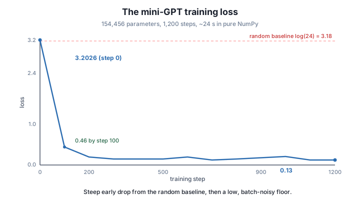
The loss starts at 3.2026, right at the random baseline of $\log(24) \approx 3.178$ we derived in Module 6: an untrained model is just guessing uniformly among the 24 characters. Within 100 steps it has collapsed to 0.46, and by step 300 it is down around 0.15, where it then hovers.

That shape — a steep early drop followed by fluctuation at a low floor — is exactly what you’d expect here. The Lantern Bay corpus is small and highly repetitive (ten sentences repeated), so there is a lot of easy structure to capture fast, and once the model has essentially learned the text the remaining loss is mostly the irreducible uncertainty at genuine branch points (after "the ", several words are plausible). The step-to-step wobble (for example the bump to 0.22 at step 1000) is batch noise: each step sees a different random batch, so the measured loss jitters even as the model is not getting worse.

Practice Exercises#

Exercise 1: Fewer steps#

Run the loop for only 100 steps and note the loss. Is 100 steps enough to get most of the way down, or does the model still have a long way to go?

Exercise 2: A bigger batch#

Change batch_size to 64 and rerun. Does the loss curve get smoother? Why would a larger batch reduce the step-to-step wobble?

Exercise 3: Track the running average#

Instead of printing the raw loss, keep an exponential moving average (avg = 0.9*avg + 0.1*loss) and print that. Why is a smoothed loss often more informative than the raw per-step value?

Summary#

A training step is four moves — batch, forward, backward, update — repeated until the model learns. Assembled from the MiniGPT, get_batch, and Adam you built, the loop trains a 154,456-parameter transformer in about 24 seconds of pure NumPy, and the loss falls from the random baseline of 3.20 to around 0.13. The steep early drop is the model capturing the corpus’s easy structure; the low-floor fluctuation is batch noise plus the irreducible uncertainty of the text.

Key Concepts#

• Training step: get_batch → forward (loss) → backward (grads) → optimizer.step.
• Loss trajectory: starts at the log(vocab_size) random baseline and falls as the model learns.
• Batch noise: per-step loss jitter caused by each step seeing a different random batch.
• Low-loss floor: on a small repetitive corpus the loss bottoms out fast, dominated by genuine branch-point uncertainty.

Why This Matters#

This four-line loop is, structurally, the same loop that trains models with hundreds of billions of parameters — only the scale of the data, the model, and the hardware differ. Seeing your own from-scratch transformer’s loss fall from the random baseline to a learned model, on a laptop, in NumPy, is the moment the architecture stops being a diagram and becomes something that demonstrably works. And having watched the raw loss wobble teaches the habit every practitioner needs: never read a single step’s number as the truth — read the trend.

Continue Building Your Skills#

Your mini-GPT now trains and its loss falls. But a falling training loss can be a trap: a model can drive its training loss down by memorizing rather than learning. The next lesson gives you the instrument that tells the difference. You’ll hold out a validation set, track train and validation loss together, and see the unmistakable signature of overfitting — the training loss falling while the validation loss climbs — along with what a learning rate set too high does to a run.