Calculate A/B Test Sample Size in Python Before You Experiment

An A/B test can run perfectly and still teach you very little. Suppose a product team compares two notification messages. The current message gets an 18% opt-in rate. The team wants to know whether a new message can raise that rate to 21%.

If the test includes only 200 visitors in each group, a real three-percentage-point change can easily be hidden by random variation. A result that is “not statistically significant” would then be hard to interpret. It might mean that the messages perform similarly, or simply that the test was too small.

This tutorial shows how to calculate the sample size before collecting data. We will plan one two-group conversion experiment in Python, compare several possible improvements, and create a power curve. This is experiment planning, not a guide to analyzing a finished A/B test.

Prerequisites and setup

You need Python 3.10 or later and basic experience running a Python file or notebook cell. You do not need previous A/B testing knowledge.

Create an isolated environment, then install the packages used here:

python -m venv .venv
source .venv/bin/activate
python -m pip install numpy scipy matplotlib

On Windows PowerShell, use .venv\Scripts\Activate.ps1 for the activation step. The published results were tested with Python 3.13.2, NumPy 2.5.1, SciPy 1.18.0, and Matplotlib 3.11.0.

Download the tutorial’s experiment planning CSV if you want the completed scenario table. It is an original synthetic dataset released under CC0-1.0. The fictional rates do not describe real users or a real product.

The mental model: four connected numbers

An A/B test sends independent visitors to two versions. Group A receives the current message, and group B receives the proposed message. An opt-in rate is a proportion: successful opt-ins divided by eligible visitors.

Sample-size planning connects four quantities:

1. The significance level, called alpha, limits the planned false-positive risk. We will use 0.05.
2. Statistical power is the probability that the planned test detects the chosen change when that change is real. We will target 0.80.
3. The effect size describes the difference we want the test to detect.
4. The sample size is the number of independent observations assigned to each group.

We know three of these values and solve for the fourth. Our baseline is 0.18, and the smallest improvement worth acting on is 0.03, so the alternative rate is 0.21. That three-point difference is the minimum detectable effect: the smallest effect used to design the test. It is a planning choice, not a promise about the final estimate.

Do not choose the detectable effect only because a larger value produces a cheaper experiment. Ask what change would be useful enough to justify a decision. Historical data can inform the baseline, but the useful change requires subject knowledge.

Put two rates on a comparable scale

The calculation uses Cohen’s h, a standardized difference between two proportions. Standardized means that the raw percentage-point difference is transformed so the power formula can work across different baseline rates.

The next function performs that transformation. asin is the inverse sine function; you do not need to calculate it by hand.

import math

def proportion_effect_size(baseline, alternative):
    return abs(
        2 * math.asin(math.sqrt(alternative))
        - 2 * math.asin(math.sqrt(baseline))
    )

effect_size = proportion_effect_size(0.18, 0.21)
print(f"Cohen's h: {effect_size:.5f}")

Cohen's h: 0.07577

The nonzero value tells us the rates differ on the transformed scale. We take the absolute value because this two-sided plan is interested in a difference in either direction. The effect size is small, which is reasonable: moving from 18% to 21% matters for this fictional decision but is not a large separation between the two rates.

The transformation matches the definition in the official statsmodels proportion effect-size documentation. We implement the short formula directly so every step remains visible.

Calculate power for one group size

Before solving for sample size, create a function that answers a simpler question: if each group has n visitors, what power does the plan have?

This tutorial uses a two-sided normal approximation for two equal, independent groups. A normal approximation uses the bell-shaped normal distribution to approximate the behavior of the test statistic. It is suitable for planning here because the expected success and failure counts are large. It is not an exact method for very small samples or very rare events.

SciPy’s norm.ppf finds the critical boundary for alpha. The cdf and sf methods calculate probability in the lower and upper tails of the normal distribution. These methods are defined in the official SciPy normal distribution reference.

from scipy.stats import norm

def approximate_power(
    sample_per_group,
    baseline,
    alternative,
    alpha=0.05,
):
    effect_size = proportion_effect_size(baseline, alternative)
    noncentrality = effect_size * math.sqrt(sample_per_group / 2)
    critical_value = norm.ppf(1 - alpha / 2)
    return float(
        norm.sf(critical_value - noncentrality)
        + norm.cdf(-critical_value - noncentrality)
    )

print(f"Power with 1,000 per group: {approximate_power(1000, 0.18, 0.21):.1%}")
print(f"Power with 3,000 per group: {approximate_power(3000, 0.18, 0.21):.1%}")

Power with 1,000 per group: 39.5%
Power with 3,000 per group: 83.5%

With 1,000 visitors per group, the planned test would detect the chosen effect only about 40% of the time. Increasing the group size to 3,000 raises power above the 80% target. More independent observations reduce uncertainty, making the same three-point difference easier to distinguish from noise.

Power is conditional. The 83.5% figure assumes the true rates are exactly 18% and 21%, the observations are independent, and the planned statistical model is appropriate. It does not mean there is an 83.5% probability that the new message is better.

Solve for the minimum whole-number sample

We could try many group sizes by hand, but a root finder can locate the point where calculated power equals 0.80. A root is an input where a function equals zero. Here, the function is calculated power - target power.

SciPy’s brentq searches inside a bracket whose ends have results on opposite sides of zero. The SciPy optimization reference lists it as a scalar root-finding method.

from scipy.optimize import brentq

def required_sample_per_group(
    baseline,
    alternative,
    target_power=0.80,
    alpha=0.05,
):
    if not 0 < baseline < 1 or not 0 < alternative < 1:
        raise ValueError("Both rates must be between 0 and 1.")
    if baseline == alternative:
        raise ValueError("The baseline and alternative rates must differ.")
    if not 0 < target_power < 1:
        raise ValueError("Target power must be between 0 and 1.")
    if not 0 < alpha < 1:
        raise ValueError("Alpha must be between 0 and 1.")

    root = brentq(
        lambda n: approximate_power(
            n, baseline, alternative, alpha
        ) - target_power,
        2,
        10_000_000,
    )
    return math.ceil(root)

sample_per_group = required_sample_per_group(0.18, 0.21)
print(f"Visitors per group: {sample_per_group:,}")
print(f"Total visitors: {2 * sample_per_group:,}")
print(f"Power after rounding: {approximate_power(sample_per_group, 0.18, 0.21):.4f}")

Visitors per group: 2,735
Total visitors: 5,470
Power after rounding: 0.8001

The root is rounded up, because a fraction of a visitor is impossible and rounding down could miss the target. The plan needs 2,735 eligible visitors in each group, or 5,470 total. At 2,734 per group, the executed calculation gives 0.79996, just below the target; at 2,735 it gives 0.80010.

This is the analyzable sample: the number of visitors whose outcomes must be available for the analysis. If some visitors will be lost because of logging failures, exclusions, or missing outcomes, increase the recruitment target separately. For example, with an expected 5% loss, divide 5,470 by 0.95 and round up to 5,758 visitors rather than treating incomplete rows as usable observations.

Compare several useful changes

A single estimate can create false confidence because the true improvement is unknown. Repeat the calculation for several minimum detectable effects while keeping the 18% baseline, 5% alpha, and 80% power fixed.

for lift_points in [1, 2, 3, 4, 5]:
    alternative = 0.18 + lift_points / 100
    n = required_sample_per_group(0.18, alternative)
    print(f"+{lift_points} point(s): {n:>6,} per group, {2*n:>6,} total")

+1 point(s): 23,665 per group, 47,330 total
+2 point(s):  6,036 per group, 12,072 total
+3 point(s):  2,735 per group,  5,470 total
+4 point(s):  1,567 per group,  3,134 total
+5 point(s):  1,020 per group,  2,040 total

The relationship is not linear. Halving the detectable change from two points to one point requires almost four times as many visitors. Small effects are difficult to separate from random variation, so precise experiments can become expensive quickly.

The chart below shows the same trade-off across a continuous range of sample sizes.

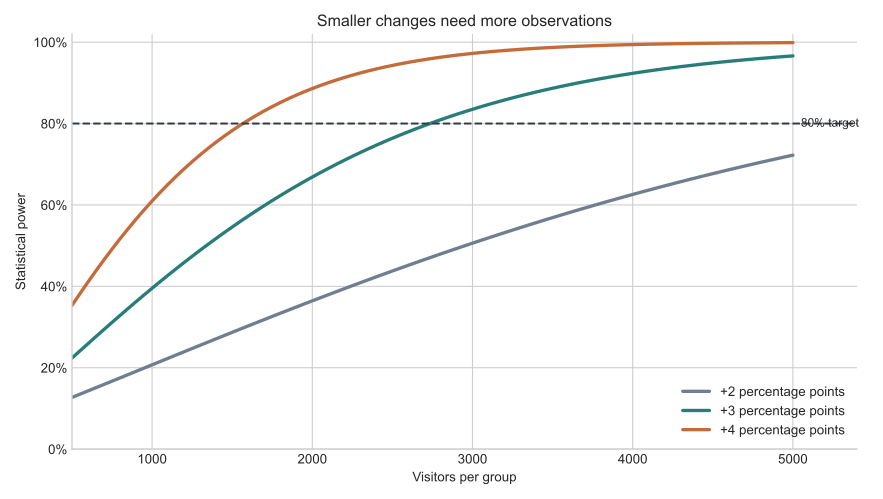
Read horizontally from the dashed 80% line to each curve, then down to the visitor count. A four-point change crosses the target earlier than a three-point change. The two-point curve has not reached 80% by 5,000 visitors per group, so its crossing lies beyond the main plotting range. A power curve helps stakeholders see the trade-off instead of treating one sample-size answer as universal.

Common mistakes and troubleshooting

Using relative lift when the code expects percentage points. Moving from 18% to 21% is a three-percentage-point increase but a 16.7% relative increase: (0.21 - 0.18) / 0.18. Pass rates 0.18 and 0.21, not 0.18 and 0.1967 unless that smaller alternative is truly your target.

Planning after looking at the result. Choosing the effect size or sample size after observing interim outcomes changes the error behavior of the test. Set the plan before launch. If you need repeated monitoring, use a method designed for sequential analysis.

Confusing power with the chance that the hypothesis is true. Power is calculated under a specific assumed alternative. It is not a posterior probability and does not tell you the probability that version B wins.

Ignoring assignment or measurement problems. More rows cannot repair duplicate users, cross-group contamination, a broken event, or a changing eligibility rule. Check the experiment design and data pipeline as carefully as the formula.

Applying the approximation to tiny expected counts. Check n * p and n * (1 - p) for both planned rates. If these expected success or failure counts are small, consult a statistician or use a method designed for sparse binary data.

Treating “no significant difference” as equality. An underpowered result does not establish that two versions are equivalent. If your real question is whether any difference is small enough to ignore, plan an equivalence or non-inferiority test with its own margin.

Recap

Sample-size planning turns an A/B testing question into four connected values: alpha, target power, a minimum detectable effect, and observations per group. For the fictional 18% versus 21% opt-in scenario, the tested normal approximation needs 2,735 visitors per group to reach about 80% power at a 5% two-sided significance level.

The durable lesson is not the number 2,735. It is the workflow: define a decision-relevant change, state the assumptions, calculate before collecting data, round up, and compare several plausible effects. Then verify assignment, tracking, and independence during the experiment. For more practice reading rates and denominators before combining them, continue with weighted averages in pandas.