Predicting Airbnb Prices: Mixing Numeric and Categorical Columns in scikit-learn

“How much should this listing cost?” is a question a host asks about one apartment, but the data that answers it never comes in one flavor. A listing’s minimum_nights is a number. Its room_type — entire home, private room, shared room — is a category. Feed both straight into LinearRegression.fit() and it crashes on the first non-numeric column it meets, because every scikit-learn estimator only ever does arithmetic.

This is where a lot of otherwise-solid tutorials quietly cheat: they either drop every non-numeric column, or one-hot encode everything by hand before the model ever sees it, which works until you need to do the exact same encoding again on new data next week. (Our post on training your first machine learning model sidesteps the problem entirely by picking a single numeric feature — a fine place to start, but real tables are rarely that polite.) This guide builds the mental model for handling mixed column types properly, then fits and honestly evaluates a price-prediction model on real, freely available Airbnb listings.

The Mental Model: Different Columns, Different Treatment, One Matrix

A LinearRegression model doesn’t actually care how many columns your table has — it cares that every value in every column is a number it can multiply by a weight. Getting there from a real table takes three steps:

1. Split the columns by type. Numeric columns (minimum_nights, availability_365, …) need one kind of treatment; categorical columns (room_type) need a completely different one.
2. Transform each group on its own terms. Numeric columns get missing values filled in and get scaled. Categorical columns get one-hot encoded — each category becomes its own 0/1 column, since there’s no honest way to multiply “Private room” by a weight.
3. Combine the transformed pieces back into one wide matrix. Every row is now all numbers, in a fixed column order, ready for .fit().

scikit-learn has one object for exactly this: ColumnTransformer. You hand it a list of (name, transformer, columns) triples, it applies each transformer to its own column subset, and it glues the results together side by side.

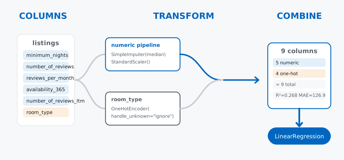
Wrap a ColumnTransformer and an estimator together in a Pipeline, and the whole three-step process becomes one object with a .fit() and a .predict() — the same shape our scikit-learn overview uses for a single preprocessing step, just with two transformers running on two different column groups instead of one.

A Dataset You Can Reproduce

Inside Airbnb publishes regularly-updated snapshots of Airbnb listings for cities around the world, released under a Creative Commons Attribution 4.0 license. Big cities like New York or London run to tens of thousands of rows — more than a tutorial needs — so this post uses a smaller market instead: Bozeman, Montana, a college and ski town with a compact, real short-term-rental scene.

Data: the Inside Airbnb Bozeman, Montana listings snapshot (CC BY 4.0), via insideairbnb.com, vendored here as a plain CSV at /datasets/blog/airbnb-price-prediction/bozeman-listings.csv, trimmed to the columns this post uses.

import pandas as pd

listings = pd.read_csv(
    "https://datatweets.com/datasets/blog/airbnb-price-prediction/bozeman-listings.csv"
)
print(listings.shape)
listings.head()

(591, 7)
         room_type  price  minimum_nights  number_of_reviews  reviews_per_month  availability_365  number_of_reviews_ltm
0  Entire home/apt  246.0               1                654               4.27               250                     87
1  Entire home/apt  407.0               2                 45               0.31               298                      6
2  Entire home/apt  267.0               2                146               1.53               227                      2
3  Entire home/apt  419.0               3                 79               0.86               274                     38
4  Entire home/apt  616.0               3                203               1.99               294                      2

Five hundred ninety-one listings, one row each: a room_type category, the nightly price we want to predict, and five numeric signals about how the listing is booked and reviewed. (The outputs in this post come from pandas 3.0 and scikit-learn 1.9 — everything shown also works on pandas 2.x and recent 1.x scikit-learn releases.)

Real Data Has Real Gaps

Before building anything, check what’s actually missing:

listings.isna().sum()

room_type                 0
price                    68
minimum_nights             0
number_of_reviews          0
reviews_per_month         75
availability_365           0
number_of_reviews_ltm      0
dtype: int64

Sixty-eight listings have no price at all — hosts who paused their listing, most likely — and 75 have no reviews_per_month, which almost certainly means “no reviews yet,” not a data-entry error. You can’t train a model to predict a target it doesn’t have, so the missing-price rows have to go. The missing reviews_per_month rows, though, still have a real price and are worth keeping — that gap gets handled inside the pipeline instead.

listings = listings.dropna(subset=["price"]).reset_index(drop=True)
print(listings.shape)
listings["room_type"].value_counts()

(523, 7)
room_type
Entire home/apt    464
Private room         46
Hotel room           10
Shared room            3
Name: count, dtype: int64

Five hundred twenty-three listings remain. Notice how lopsided room_type is: entire homes outnumber shared rooms more than 150 to 1. Keep that number in mind — it’s the reason the second gotcha below exists.

Splitting Before You Touch Anything

The features split into two groups by type, and the split into train and test happens before any transformer sees the data — fitting a scaler or encoder on data that includes the test set is a subtle way of letting the model peek at answers it shouldn’t have yet:

from sklearn.model_selection import train_test_split

numeric_features = ["minimum_nights", "number_of_reviews", "reviews_per_month", "availability_365", "number_of_reviews_ltm"]
categorical_features = ["room_type"]

X = listings[numeric_features + categorical_features]
y = listings["price"]

X_train, X_test, y_train, y_test = train_test_split(X, y, test_size=0.2, random_state=42)
print(X_train.shape, X_test.shape)

(418, 6) (105, 6)

Four hundred eighteen listings to learn from, 105 held back to grade the model honestly at the end.

Building the ColumnTransformer and Pipeline

Now the mental model becomes code. The numeric columns get their own two-step pipeline — fill missing values with the column median, then scale — and the categorical column gets OneHotEncoder. ColumnTransformer runs both and stitches the results together; wrapping it in a Pipeline with LinearRegression gives one object that does preprocessing and modeling in a single .fit() call. (The full option list for both objects is in scikit-learn’s ColumnTransformer and Pipeline user guide.)

from sklearn.compose import ColumnTransformer
from sklearn.pipeline import Pipeline
from sklearn.impute import SimpleImputer
from sklearn.preprocessing import OneHotEncoder, StandardScaler
from sklearn.linear_model import LinearRegression

numeric_pipeline = Pipeline([
    ("impute", SimpleImputer(strategy="median")),
    ("scale", StandardScaler()),
])

preprocessing = ColumnTransformer([
    ("numeric", numeric_pipeline, numeric_features),
    ("category", OneHotEncoder(handle_unknown="ignore"), categorical_features),
])

model = Pipeline([
    ("preprocessing", preprocessing),
    ("regressor", LinearRegression()),
])

model.fit(X_train, y_train)

Nothing prints from a successful .fit(), but you can ask the fitted ColumnTransformer exactly what it built:

model.named_steps["preprocessing"].get_feature_names_out()

['numeric__minimum_nights' 'numeric__number_of_reviews'
 'numeric__reviews_per_month' 'numeric__availability_365'
 'numeric__number_of_reviews_ltm' 'category__room_type_Entire home/apt'
 'category__room_type_Hotel room' 'category__room_type_Private room'
 'category__room_type_Shared room']

Five numeric columns went in unchanged in name (just imputed and scaled); one categorical column came out as four — one 0/1 column per category OneHotEncoder saw during .fit(). That’s the “combine” step from the mental model, made concrete: nine columns, all numbers, one matrix.

Grading the Model Honestly

LinearRegression never saw the test set during .fit(), so predicting on it is a fair test:

from sklearn.metrics import mean_absolute_error, r2_score

preds = model.predict(X_test)
print("R2:", round(r2_score(y_test, preds), 3))
print("MAE:", round(mean_absolute_error(y_test, preds), 2))

R2: 0.268
MAE: 126.9

Read this honestly rather than hopefully: an R² of 0.268 means these five booking signals and the room type explain roughly a quarter of the variation in price — real predictive signal, but nowhere near enough to price a listing on their own. The average prediction misses by about $127. That’s not a failure of the code; it’s an accurate report that nightly price depends heavily on things this dataset doesn’t capture, like square footage, amenities, and exact location. A model that reported a suspiciously high R² on a table this thin would be the thing to distrust, not celebrate.

The fitted coefficients tell you which signals pulled in which direction:

coefs = model.named_steps["regressor"].coef_
names = model.named_steps["preprocessing"].get_feature_names_out()
for n, c in zip(names, coefs):
    print(f"{n}: {c:.2f}")

numeric__minimum_nights: -97.61
numeric__number_of_reviews: -24.17
numeric__reviews_per_month: -42.81
numeric__availability_365: 9.09
numeric__number_of_reviews_ltm: 37.52
category__room_type_Entire home/apt: 186.54
category__room_type_Hotel room: -66.94
category__room_type_Private room: 34.23
category__room_type_Shared room: -153.83

Because every numeric column was scaled first, these coefficients are roughly comparable to each other: a longer required minimum stay and a heavier recent review pace both pull price down (short, popular stays behave differently from long-term rentals here), while entire homes command a clear premium over every other room type.

Three Gotchas Worth Knowing

A category your training data never saw will crash a strict encoder — handle_unknown="ignore" is not optional for lopsided categories. With room_type split roughly 150-to-1 in favor of entire homes, an unlucky train/test split can leave a rare category like “Shared room” entirely out of the training rows:

X_train6, X_test6 = train_test_split(X[["room_type"]], test_size=0.2, random_state=6)
print("train categories:", sorted(X_train6["room_type"].unique()))
print("test categories: ", sorted(X_test6["room_type"].unique()))

from sklearn.preprocessing import OneHotEncoder

strict_encoder = OneHotEncoder(handle_unknown="error").fit(X_train6)
strict_encoder.transform(X_test6)

train categories: ['Entire home/apt', 'Hotel room', 'Private room']
test categories:  ['Entire home/apt', 'Hotel room', 'Private room', 'Shared room']
ValueError: Found unknown categories ['Shared room'] in column 0 during transform

With the default handle_unknown="error", that’s a hard crash the moment real test (or production) data shows up with a category the encoder never learned. Swap in handle_unknown="ignore" and the same unseen category quietly becomes all zeros across the known columns instead of raising:

safe_encoder = OneHotEncoder(handle_unknown="ignore").fit(X_train6)
encoded_test = safe_encoder.transform(X_test6).toarray()
shared_row = X_test6.reset_index(drop=True).query("room_type == 'Shared room'").index[0]
print("encoded categories:", list(safe_encoder.categories_[0]))
print("a Shared room row encodes as:", encoded_test[shared_row])

encoded categories: ['Entire home/apt', 'Hotel room', 'Private room']
a Shared room row encodes as: [0. 0. 0.]

That all-zero row isn’t a special “unknown” flag — it’s just a listing that doesn’t match any category the model learned about, so it contributes nothing extra beyond the intercept and the numeric features. Worth knowing, not necessarily worth celebrating.

How you fill in missing values changes the fitted model, even when the accuracy barely moves. reviews_per_month was missing for listings with no reviews yet. Filling it with the column median versus filling it with a flat 0 are different, defensible choices with different downstream numbers:

numeric_pipeline_zero = Pipeline([
    ("impute", SimpleImputer(strategy="constant", fill_value=0)),
    ("scale", StandardScaler()),
])
preprocessing_zero = ColumnTransformer([
    ("numeric", numeric_pipeline_zero, numeric_features),
    ("category", OneHotEncoder(handle_unknown="ignore"), categorical_features),
])
model_zero = Pipeline([("preprocessing", preprocessing_zero), ("regressor", LinearRegression())])
model_zero.fit(X_train, y_train)
preds_zero = model_zero.predict(X_test)

print("MAE median-impute:", round(mean_absolute_error(y_test, preds), 2))
print("MAE zero-impute:  ", round(mean_absolute_error(y_test, preds_zero), 2))

MAE median-impute: 126.9
MAE zero-impute:   128.63

The gap here is small, but it won’t always be. Zero-filling silently claims “no reviews yet” behaves like “reviews every month,” which is a real (if minor) modeling assumption baked in by one keyword argument — decide it on purpose, don’t let the default happen to you.

Fitting a scaler before you split leaks test-set statistics into training. StandardScaler learns a mean and standard deviation from whatever it’s fitted on. Fit it on the full 523 rows and those statistics quietly include information from the 105 rows you meant to hold out:

import numpy as np
from sklearn.preprocessing import StandardScaler

leaky_scaler = StandardScaler().fit(X[numeric_features].fillna(X[numeric_features].median()))
honest_scaler = StandardScaler().fit(X_train[numeric_features].fillna(X_train[numeric_features].median()))

print("mean fit on all 523 rows:  ", np.round(leaky_scaler.mean_, 2))
print("mean fit on train 418 rows:", np.round(honest_scaler.mean_, 2))

mean fit on all 523 rows:   [  9.6   90.45   1.83 229.68  17.38]
mean fit on train 418 rows: [  9.43  92.94   1.87 229.14  17.74]

The difference looks tiny on 523 rows split one way, but the direction of the mistake is always the same: your reported test score gets a little too optimistic, in a way that won’t reproduce once real, truly-unseen data shows up. This is also the strongest argument for putting the scaler inside the Pipeline in the first place — call .fit() on X_train alone, as this post did, and the leak can’t happen by accident.

Wrapping Up

Mixed column types aren’t an edge case — they’re what real tables look like. The pattern that handles them:

• ColumnTransformer → routes each column group to its own transformer (impute-and-scale for numbers, OneHotEncoder for categories)
• Pipeline → chains that preprocessing with an estimator into one .fit()/.predict() object
• handle_unknown="ignore" → keeps a lopsided category from crashing your encoder on a bad split or on production data
• Split first, fit second → the only way to grade a model honestly and keep test-set statistics out of training

If you want to build on this with a full regression workflow — reading standardized coefficients, checking model fit, and validating on a real project — the Regression module in our free Machine Learning course picks up exactly where this post’s preprocessing leaves off.