How to Analyze Survey Data in Python: Percentages, Crosstabs, Chi-Square

Say you’ve got 1,040 filled-out survey responses in a CSV. Someone is going to ask you what people actually think, and “58% said no” is rarely the whole answer they need — they want to know whether that 58% holds up once you split the room by who’s answering, and whether the split you’re seeing is a real pattern or just how this particular batch of 1,040 people happened to land. Getting from a loaded DataFrame to an answer you’d defend in a meeting is a smaller jump than it looks, and it doesn’t require anything beyond pandas and one function from scipy.

If your CSV itself is the problem — a two-row header, “select all that apply” columns, a forced-rank question stored as six numeric columns — that’s a separate fight, and our post on wrangling survey data with pandas covers it in depth. This post assumes you’re past that stage: one column per question, and now you need real numbers out of it. In short, that means running value_counts(normalize=True) per question instead of trusting raw counts, cross-tabulating a question against a group with pd.crosstab(..., normalize="index") to compare, and treating a group difference as real only once a chi-square test on the underlying counts (scipy.stats.chi2_contingency) backs it up.

Count, Compare, Confirm: The Shape of a Survey Analysis

Nearly every question someone asks about survey results reduces to one of three moves, done in order.

1. Count. What share of respondents picked each answer? This is a frequency table — one question, one distribution.
2. Compare. Does that distribution look different across a group — men versus women, frequent flyers versus occasional ones, one region versus another? This is a cross-tabulation — two questions, one table.
3. Confirm. Is that difference big enough to trust, or small enough that a different batch of 1,040 respondents could have shown the opposite? This is a significance test — a yes-or-no check on the table from step two.

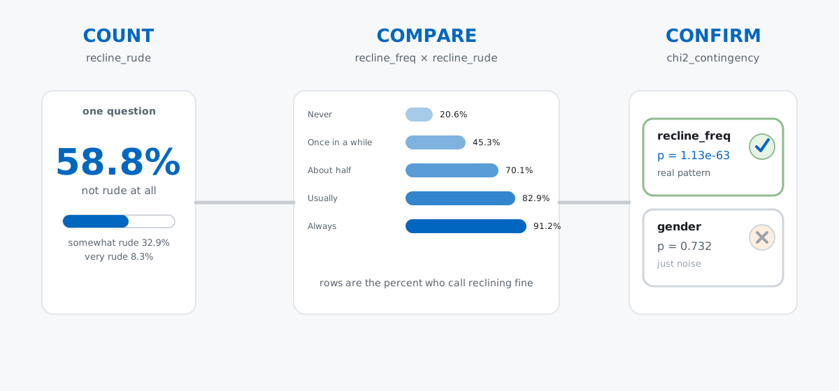
Skipping straight to “confirm” without doing “compare” first is how people end up running a statistical test on a question that never needed one. Skipping “confirm” after “compare” is how a difference that’s really just noise gets reported as a finding. We’ll walk all three, in order, on one real dataset.

The Survey: 1,040 Readers on Airplane Etiquette

FiveThirtyEight ran a reader survey in 2014 asking about the unwritten rules of flying: whether it’s rude to recline your seat, who gets the armrest, whether it’s okay to wake a stranger to get to the bathroom. It’s a good fit here because the questions are opinions with real disagreement behind them, and the file ships with enough demographics (gender, age, region) to make genuine comparisons.

Data: FiveThirtyEight’s 2014 “Flying Etiquette” survey (CC BY 4.0), via FiveThirtyEight’s public data repository. Grab a copy at /datasets/blog/analyze-survey-data-python/flying-etiquette.csv to follow along with the numbers below.

import pandas as pd
from scipy.stats import chi2_contingency

survey_raw = pd.read_csv("flying-etiquette.csv")
survey_raw.shape

(1040, 27)

Twenty-seven columns, most named after the full question text. We only need a handful for this post, so pull those out and give them names you can actually type:

columns = {
    "How often do you travel by plane?": "travel_freq",
    "Do you ever recline your seat when you fly?": "recline_freq",
    "Is itrude to recline your seat on a plane?": "recline_rude",
    "Gender": "gender",
    "Location (Census Region)": "region",
}
survey = survey_raw[list(columns)].rename(columns=columns)
survey["travel_freq"].value_counts(dropna=False)

travel_freq
Once a year or less      633
Once a month or less     205
Never                    166
A few times per month     29
A few times per week       4
Every day                  3
Name: count, dtype: int64

166 respondents said they never fly, and the questionnaire’s own skip logic left every reclining-related column blank for them — they were never asked. (That’s the same skip logic vs. real nonresponse distinction our Star Wars survey post digs into; here we just need to filter it out.) Keep only people who actually fly:

flyers = survey[survey["travel_freq"] != "Never"].copy()
flyers.shape

(874, 5)

874 people who fly, five columns, ready for the count-compare-confirm sequence. (The outputs in this post come from pandas 3.0.3 and scipy 1.18.0.)

Percentages, Not Just Counts

The “count” step starts with a single question: is it rude to recline your seat?

flyers["recline_rude"].value_counts(dropna=False)

recline_rude
No, not rude at all    502
Yes, somewhat rude     281
Yes, very rude          71
NaN                     20
Name: count, dtype: int64

Raw counts don’t tell you much on their own — 502 out of what? value_counts() drops NaN by default, so the plain-percentage version answers that automatically, out of the 854 people who actually answered:

flyers["recline_rude"].value_counts(normalize=True).round(3)

recline_rude
No, not rude at all    0.588
Yes, somewhat rude     0.329
Yes, very rude         0.083
Name: proportion, dtype: float64

58.8% call it not rude at all. That’s the number a headline would use, and it’s not wrong — but it’s an average over everyone, and averages over everyone hide whatever’s driving the opinion in the first place. Before comparing anything, drop the stragglers who left either reclining question blank, so every later table is built on the same set of people:

flyers = flyers.dropna(subset=["recline_freq", "recline_rude"]).copy()
flyers.shape

(854, 5)

Keeping an Opinion Scale in Its Real Order

recline_freq is a frequency scale — Never, Once in a while, About half the time, Usually, Always — and pandas has no way to know that on its own:

flyers["recline_freq"].value_counts(normalize=True).round(3)

recline_freq
Once in a while        0.300
Usually                0.205
Never                  0.199
Always                 0.159
About half the time    0.137
Name: proportion, dtype: float64

That ordering is alphabetical, which scrambles a scale that’s supposed to read low-to-high. Tell pandas the real order with an ordered Categorical, and both sorting and later comparisons respect it:

recline_order = ["Never", "Once in a while", "About half the time", "Usually", "Always"]
flyers["recline_freq"] = pd.Categorical(flyers["recline_freq"], categories=recline_order, ordered=True)
flyers["recline_freq"].value_counts(normalize=True).sort_index().round(3)

recline_freq
Never                  0.199
Once in a while        0.300
About half the time    0.137
Usually                0.205
Always                 0.159
Name: proportion, dtype: float64

Same five numbers, but sort_index() now walks Never through Always in the order a human would read them, and any later groupby or crosstab on this column will do the same. Do this for recline_rude too — it’s a three-point rudeness scale, and the same trap applies:

rude_order = ["No, not rude at all", "Yes, somewhat rude", "Yes, very rude"]
flyers["recline_rude"] = pd.Categorical(flyers["recline_rude"], categories=rude_order, ordered=True)

Cross-Tabulating an Opinion Against a Behavior

Here’s the “compare” step: does how often someone reclines predict whether they think reclining is rude? pd.crosstab builds the joint frequency table, and normalize="index" turns each row into percentages that sum to 100 — “of the people at this reclining frequency, what did they say about rudeness”:

ct = pd.crosstab(flyers["recline_freq"], flyers["recline_rude"], normalize="index") * 100
ct.round(1)

recline_rude         No, not rude at all  Yes, somewhat rude  Yes, very rude
recline_freq                                                                
Never                               20.6                47.6            31.8
Once in a while                     45.3                50.4             4.3
About half the time                 70.1                29.9             0.0
Usually                             82.9                15.4             1.7
Always                              91.2                 6.6             2.2

That’s about as clean a self-serving-bias result as survey data produces: 20.6% of people who never recline think it’s fine, versus 91.2% of people who always do. Nobody’s lying — people who recline every flight have simply had more chances to convince themselves it’s fine, and people who never recline have had more chances to be annoyed by someone else’s seatback. The overall 58.8% from the count step was quietly averaging over both ends of a 70-point spread.

Is That Difference Real? A Chi-Square Test

A 70-point spread across five groups of unequal size is where “confirm” earns its place: is that pattern too big to be an artifact of who happened to answer this particular survey? scipy.stats.chi2_contingency takes the raw counts (not the percentages) and tests whether reclining frequency and rudeness opinion are independent:

ct_counts = pd.crosstab(flyers["recline_freq"], flyers["recline_rude"])
chi2, p, dof, expected = chi2_contingency(ct_counts)
print(f"chi2={chi2:.1f} dof={dof} p={p:.2e}")

chi2=316.7 dof=8 p=1.13e-63

A p-value that small isn’t really “1.13 times ten to the minus 63” in any meaningful sense — it’s “essentially zero, far past any threshold you’d ever need.” If reclining frequency and rudeness opinion were truly unrelated, seeing a table this lopsided by chance is not a realistic possibility. This one’s genuinely useful to test, because the raw table already made the pattern obvious. Run the same test on a split that doesn’t obviously matter, and the test earns its keep the other way:

flyers_g = flyers.dropna(subset=["gender"]).copy()
ctg_counts = pd.crosstab(flyers_g["gender"], flyers_g["recline_rude"])
ctg_pct = pd.crosstab(flyers_g["gender"], flyers_g["recline_rude"], normalize="index") * 100
print(ctg_pct.round(1))
chi2g, pg, dofg, _ = chi2_contingency(ctg_counts)
print(f"chi2={chi2g:.3f} dof={dofg} p={pg:.3f}")

recline_rude  No, not rude at all  Yes, somewhat rude  Yes, very rude
gender                                                               
Female                       58.4                33.9             7.7
Male                         58.9                32.2             9.0

chi2=0.625 dof=2 p=0.732

58.4% versus 58.9% — a gap that small could easily flip the other way in a second survey, and p=0.732 says exactly that: nowhere near the threshold where you’d call it a real difference. Gender isn’t the story here; reclining frequency is. That’s the actual value of the confirm step — not to bless every crosstab you build, but to tell you which ones deserve a sentence in your write-up and which ones are noise dressed up as a finding.

Where Survey Percentages Go Wrong

normalize="index" and normalize="columns" answer different questions, and mixing them up produces a table that looks right and means the opposite thing. normalize="index" (used above) answers “of people at this reclining frequency, what fraction hold each opinion” — each row sums to 100. Ask for normalize="columns" instead and you get “of people who hold each opinion, what fraction recline at this frequency” — each column sums to 100:

pd.crosstab(flyers["recline_freq"], flyers["recline_rude"], normalize="columns").round(3) * 100

recline_rude         No, not rude at all  Yes, somewhat rude  Yes, very rude
recline_freq                                                                
Never                                7.0                28.8            76.1
Once in a while                     23.1                45.9            15.5
About half the time                 16.3                12.5             0.0
Usually                             28.9                 9.6             4.2
Always                              24.7                 3.2             4.2

Read that “Never” row now and it says 76.1% — not 20.6%. Nothing changed except which axis got forced to 100; both numbers are correct answers to different questions, and picking the wrong one for your sentence is an easy way to accidentally reverse a claim.

Small subgroups turn noise into a headline. Census region breaks the 854 respondents into nine groups, and they aren’t close to the same size:

flyers.dropna(subset=["region"]).groupby("region", observed=True).size().sort_values()

region
East South Central     25
Mountain               54
New England            55
West North Central     66
West South Central     81
Middle Atlantic       111
East North Central    122
South Atlantic        138
Pacific               185
dtype: int64

East South Central’s 25 respondents produce a “not rude at all” rate of 64.0%, versus New England’s 55 respondents at 69.1% — a five-point gap that looks like a regional story. But with only 25 people, two of them changing their answer moves that percentage by 8 points; the same two people would barely register against Pacific’s 185. Before you trust a regional (or any small-group) difference, check the denominator it’s built on.

A significant p-value describes this sample, not the population it came from. FiveThirtyEight recruited these 1,040 respondents online — through their own readership, not a random sample of the flying public — so even a chi-square result as decisive as p=1.13e-63 only tells you the pattern is unlikely to be a fluke of this specific batch of respondents. It doesn’t promote “58.8% of Americans” to a fact about Americans. That distinction matters every time a convenience-sample survey (which is most of them, including internal customer or employee surveys) gets summarized as if it were a poll of the whole population.

The Same Three Steps, Any Survey

Count gave an honest baseline (58.8% don’t find reclining rude); compare split it by reclining frequency and found the real story (20.6% to 91.2%); confirm checked that story against chance and ruled it in (p=1.13e-63) while ruling gender out (p=0.732). That sequence doesn’t change from survey to survey — only the questions and the groups do.

If you want the statistical backbone behind the confirm step — contingency tables, expected counts, and what the chi-square statistic is actually measuring — the Chi-Squared Test of Independence lesson in our free Statistics & Probability course works through it on two more datasets with the same rigor applied here.