Exploratory Data Analysis with Pandas: A Video Game Dataset Walkthrough

You just got handed a CSV you’ve never seen before. Before you can plot anything, filter anything, or answer whatever question made someone hand it to you in the first place, you have to answer a smaller, quieter one: what actually is this data? How many rows, what columns, what’s typical, what’s weird? That’s exploratory data analysis (EDA) — not a single method, but the first-pass routine you run on any new dataset before you trust it.

Most pandas tutorials teach EDA as a grab bag of unrelated methods — here’s .info(), here’s .describe(), here’s .groupby() — without ever showing how they chain together into one investigation. That’s where people stall out: they know the individual tools but not the order to reach for them in. This guide gives you that order as a repeatable process, then runs it start to finish on a small dataset you can regenerate exactly. If you want a deeper dive into .groupby() itself once you’re past the first pass — agg, transform, filter — our pandas GroupBy guide picks up exactly where this post’s groupby section leaves off.

The Mental Model: Shape, Summary, Questions, Answers

Every first pass at a new dataset is the same four moves, in the same order:

1. Shape. How big is this, and what’s in each column? Row count, column count, and dtypes — before you trust a single number, know what kind of thing it is.
2. Summary. What does “typical” look like? A quick statistical fingerprint of every column, numeric and categorical, so outliers and surprises show up before you go looking for them.
3. Questions. Turn curiosity into code. “What’s the best X in category Y?” becomes a filter plus a sort.
4. Answers, per group. Most real questions aren’t about one row, they’re about a category — average by genre, count by year. That’s .groupby().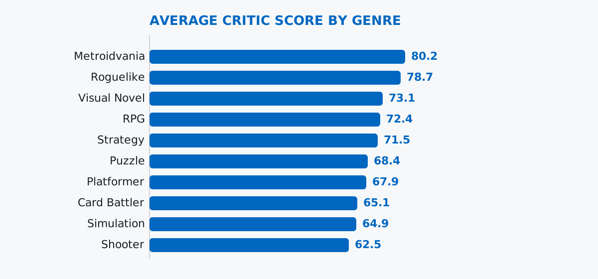

That chart is the answer this post arrives at by the end — proof that “shape, summary, questions, answers” isn’t an abstract idea, it’s a path you can actually walk to a real result. Keep the four steps in mind; the rest of this post just is those steps, in order, on one dataset.

A Dataset You Can Reproduce

Imagine you’ve just joined the small team behind Driftwood Arcade, a boutique digital storefront that publishes indie games from dozens of small studios. Someone hands you the full release catalog — every game they’ve ever published, since the label launched in 2014 — and asks, essentially, “so what’s in here?” That’s the scenario for this post.

Driftwood Arcade is invented for this tutorial, and so is its catalog: titles, genres, platforms, review scores, and playtime are all generated with a fixed random seed, so your numbers will match mine exactly. Real “video game sales” datasets circulating online are almost all scraped from a single sales-estimate site whose own terms don’t actually permit redistribution, no matter what license a re-upload claims — so this post sidesteps that risk entirely with an original, synthetic catalog instead.

import numpy as np
import pandas as pd

rng = np.random.default_rng(42)
n = 400

genres = ["Platformer", "Puzzle", "RPG", "Roguelike", "Shooter",
          "Simulation", "Strategy", "Visual Novel", "Metroidvania", "Card Battler"]
genre_p = [0.14, 0.11, 0.10, 0.09, 0.09, 0.09, 0.09, 0.10, 0.10, 0.09]

platforms = ["Windows", "macOS", "Switch", "PlayStation", "Xbox"]
platform_p = [0.34, 0.14, 0.24, 0.15, 0.13]

genre_score_bias = {
    "Platformer": 68, "Puzzle": 71, "RPG": 74, "Roguelike": 78, "Shooter": 63,
    "Simulation": 66, "Strategy": 70, "Visual Novel": 73, "Metroidvania": 80,
    "Card Battler": 69,
}
genre_hours_bias = {
    "Platformer": 6, "Puzzle": 4, "RPG": 28, "Roguelike": 18, "Shooter": 8,
    "Simulation": 22, "Strategy": 20, "Visual Novel": 9, "Metroidvania": 12,
    "Card Battler": 15,
}

adjectives = ["Hollow", "Brass", "Salt", "Ember", "Nine", "Quiet", "Iron", "Static",
              "Faded", "Copper", "Wandering", "Sunken", "Velvet", "Broken", "Amber",
              "Last", "Pale", "Rusted", "Dim", "Tangled"]
nouns = ["Orchard", "Vector", "Harbor", "Atlas", "Chorus", "Ridge", "Foundry",
         "Meridian", "Warren", "Lantern", "Circuit", "Thicket", "Anchor",
         "Signal", "Verge", "Reef", "Bastion", "Current", "Loom", "Cinder"]
combos = [f"{a} {b}" for a in adjectives for b in nouns]
titles = rng.choice(combos, size=n, replace=False)

genre = rng.choice(genres, size=n, p=genre_p)
platform = rng.choice(platforms, size=n, p=platform_p)
release_year = rng.integers(2014, 2027, size=n)
price_usd = rng.choice([4.99, 9.99, 14.99, 19.99, 24.99, 29.99], size=n,
                        p=[0.12, 0.28, 0.27, 0.18, 0.10, 0.05])

base_score = np.array([genre_score_bias[g] for g in genre], dtype=float)
critic_score = np.clip(base_score + rng.normal(0, 8, size=n), 20, 100).round(1)

base_rating = critic_score / 100 * 5
user_rating = np.clip(base_rating + rng.normal(0, 0.4, size=n), 0, 5).round(1)
missing_mask = (release_year == 2026) & (rng.random(n) < 0.55)
missing_mask |= rng.random(n) < 0.03
user_rating = user_rating.astype(float)
user_rating[missing_mask] = np.nan

base_hours = np.array([genre_hours_bias[g] for g in genre], dtype=float)
playtime_hours = rng.lognormal(mean=np.log(base_hours), sigma=0.35, size=n).round(1)

games = pd.DataFrame({
    "title": titles,
    "genre": genre,
    "platform": platform,
    "release_year": release_year,
    "price_usd": price_usd,
    "critic_score": critic_score,
    "user_rating": user_rating,
    "playtime_hours": playtime_hours,
})

games.head()

            title         genre     platform  release_year  price_usd  critic_score  user_rating  playtime_hours
0  Velvet Current       Shooter       Switch          2017       9.99          76.7          4.0             5.5
1     Last Chorus           RPG  PlayStation          2023      14.99          92.1          4.3            15.8
2  Copper Lantern  Card Battler      Windows          2014       4.99          60.8          3.3            13.3
3   Static Harbor  Visual Novel         Xbox          2021      29.99          73.6          3.4            11.8
4    Faded Cinder    Platformer       Switch          2023       9.99          58.6          2.7            10.8

400 games, 8 columns, one row per title. (The outputs in this post come from pandas 3.0.3 — everything shown also works on pandas 2.x.)

Step 1, Shape: .shape, .dtypes, and .info()

Before anything else, how big is this and what’s in it:

games.shape

(400, 8)

games.dtypes

title                 str
genre                 str
platform              str
release_year        int64
price_usd         float64
critic_score      float64
user_rating       float64
playtime_hours    float64
dtype: object

.shape gives you the two numbers that anchor everything else — 400 rows, 8 columns — and .dtypes tells you what kind of column you’re dealing with before you try to do math on it. .info() combines both, plus something neither one shows on its own: how many values are actually present in each column.

games.info()

<class 'pandas.DataFrame'>
RangeIndex: 400 entries, 0 to 399
Data columns (total 8 columns):
 #   Column          Non-Null Count  Dtype  
---  ------          --------------  -----  
 0   title           400 non-null    str    
 1   genre           400 non-null    str    
 2   platform        400 non-null    str    
 3   release_year    400 non-null    int64  
 4   price_usd       400 non-null    float64
 5   critic_score    400 non-null    float64
 6   user_rating     368 non-null    float64
 7   playtime_hours  400 non-null    float64
dtypes: float64(4), int64(1), str(3)
memory usage: 25.1 KB

Read the Non-Null Count column right away: user_rating has 368, not 400 — 32 games have no recorded player rating yet, which makes sense for a catalog that includes very recent releases. This post keeps that gap as-is rather than filling or dropping it, since it doesn’t block anything below; if you want the fuller playbook for deciding what to do with a gap like this — fill it, drop it, or leave it — our guide to cleaning messy data with pandas is the deeper dive.

Step 2, Summary: .describe() for a First Numeric Read

.describe() is the fastest way to get a statistical fingerprint of every numeric column at once:

games.describe()

       release_year   price_usd  critic_score  user_rating  playtime_hours
count    400.000000  400.000000    400.000000   368.000000       400.00000
mean    2019.967500   15.527500     70.390000     3.522826        14.34400
std        3.843615    6.699687      9.337434     0.625150         9.69022
min     2014.000000    4.990000     41.600000     1.400000         1.60000
25%     2017.000000    9.990000     64.475000     3.100000         6.70000
50%     2020.000000   14.990000     70.200000     3.500000        11.80000
75%     2023.250000   19.990000     75.925000     3.900000        19.50000
max     2026.000000   29.990000     99.600000     5.000000        55.20000

Read each column top to bottom: count confirms what .info() already told you (368 for user_rating, 400 everywhere else), mean and 50% (the median) give you two different ideas of “typical,” and min/max bound the range — a critic score as low as 41.6 and as high as 99.6 tells you this catalog has real quality spread, not everything clustered near one number. The pandas user guide’s essential basic functionality page documents .describe() and the rest of this summary toolkit in full, including how to compute individual pieces like .mean() or .quantile() on their own.

Notice what’s missing from that table: title, genre, and platform — the three text columns — aren’t there at all. More on that in the gotchas section below.

Step 3, Questions: Filtering and Sorting to Get an Answer

Summaries describe the whole dataset; a real question is usually narrower. Say you want to know: what are the highest-rated Roguelike games in the catalog?

roguelikes = games[games["genre"] == "Roguelike"]
top_roguelikes = roguelikes.sort_values("critic_score", ascending=False).head(5)
top_roguelikes[["title", "platform", "release_year", "critic_score"]]

        title    platform  release_year  critic_score
 Quiet Warren PlayStation          2025          99.6
 Tangled Reef PlayStation          2016          90.5
 Copper Ridge PlayStation          2019          89.4
Amber Foundry      Switch          2020          85.0
 Iron Circuit       macOS          2018          85.0

Two steps, in order: games["genre"] == "Roguelike" builds a boolean mask that keeps only Roguelike rows, then .sort_values("critic_score", ascending=False) puts the highest scores first. .head(5) just trims the result to a readable size. This is the pattern behind almost any “what’s the best/worst/most/least X” question — filter down to the rows that matter, then sort by the number you care about.

Step 4, Answers Per Group: .groupby() for a Summary View

A single top-5 list answers one question about one genre. The more useful question is usually about every genre at once — which is exactly what .groupby() is for:

avg_score_by_genre = games.groupby("genre")["critic_score"].mean().round(1).sort_values(ascending=False)
avg_score_by_genre

genre
Metroidvania    80.2
Roguelike       78.7
Visual Novel    73.1
RPG             72.4
Strategy        71.5
Puzzle          68.4
Platformer      67.9
Card Battler    65.1
Simulation      64.9
Shooter         62.5
Name: critic_score, dtype: float64

That’s a full summary of the catalog by genre in one line: split the rows by genre, average critic_score within each group, sort the results. Metroidvania games score highest on average in this catalog, Shooters lowest — a genre-level pattern that no single row could have shown you. Adding a second and third metric to the same summary is just as short with named aggregations:

genre_summary = games.groupby("genre").agg(
    avg_score=("critic_score", "mean"),
    avg_hours=("playtime_hours", "mean"),
    n_games=("title", "count"),
).round(1).sort_values("avg_score", ascending=False)
genre_summary

              avg_score  avg_hours  n_games
genre                                      
Metroidvania       80.2       14.2       40
Roguelike          78.7       20.3       30
Visual Novel       73.1       10.0       41
RPG                72.4       29.4       42
Strategy           71.5       20.1       38
Puzzle             68.4        4.5       43
Platformer         67.9        6.2       65
Card Battler       65.1       16.1       34
Simulation         64.9       23.4       31
Shooter            62.5        7.9       36

Now the top-scoring genres come with context: Metroidvania and Roguelike titles don’t just score well, they also run long (14.2 and 20.3 hours on average) — while Puzzle games score respectably at 68.4 but average only 4.5 hours, a completely different kind of catalog entry. n_games matters too: with only 30 Roguelike titles behind that 78.7 average, it’s a smaller sample than the 65 Platformer games sitting at 67.9. (For the full toolkit here — agg, transform, filter, multi-column grouping — the pandas GroupBy guide covers it end to end.)

Step 4, Continued: Turning the Groupby into a Chart

A sorted table already reads well, but a chart makes the size of the gap between genres immediate:

import matplotlib
matplotlib.use("Agg")
import matplotlib.pyplot as plt

fig, ax = plt.subplots(figsize=(7, 4))
avg_score_by_genre.sort_values().plot(kind="barh", ax=ax, color="#0067c0")
ax.set_xlabel("average critic score")
ax.set_title("Average critic score by genre")
fig.tight_layout()

print("bars:", len(ax.patches))
print([round(p.get_width(), 1) for p in ax.patches])

bars: 10
[62.5, 64.9, 65.1, 67.9, 68.4, 71.5, 72.4, 73.1, 78.7, 80.2]

Series.plot(kind="barh") reads the Series you already built — index as category labels, values as bar lengths — and hands back an ordinary matplotlib Axes, the same object plt.subplots() gives you directly. The ten bar widths printed above are exactly the ten averages from avg_score_by_genre, just confirmed programmatically instead of eyeballed, since this post’s verification runs headlessly rather than opening a window. The diagram at the top of this post is this same chart, redrawn in the site’s house style with the same numbers.

Three Gotchas Worth Knowing

.describe() silently drops non-numeric columns unless you ask for them back. Run it plain and title, genre, and platform just aren’t there — no error, no warning, they’re simply gone:

games.describe().columns.tolist()

['release_year', 'price_usd', 'critic_score', 'user_rating', 'playtime_hours']

games.describe(include="all").columns.tolist()

['title', 'genre', 'platform', 'release_year', 'price_usd', 'critic_score', 'user_rating', 'playtime_hours']

include="all" brings every column back, text ones included — though for text columns you get count, unique, top, and freq instead of a mean or a percentile, since those don’t mean anything for a genre name. If you only ever run the plain version, it’s easy to forget you have three whole columns .describe() never showed you.

.sort_values() defaults to ascending — “sorted” doesn’t mean “best first.” Sort by critic_score with no other arguments and you get the worst games at the top, not the best:

games.sort_values("critic_score").head(3)[["title", "genre", "critic_score"]]

         title      genre  critic_score
Static Thicket Simulation          41.6
  Quiet Vector    Shooter          45.8
  Brass Cinder Platformer          47.2

You need ascending=False for “highest first,” the same argument used in every ranking example earlier in this post. It’s an easy one to forget under deadline pressure, and the bug is silent — the code runs fine, it just answers the opposite question from the one you meant to ask.

Filtering doesn’t renumber the index — a label-based lookup can break even though a positional one won’t. Filter down to premium-priced games and the surviving rows keep their original row labels, not a fresh 0, 1, 2, ...:

premium = games[games["price_usd"] >= 24.99]
premium.index[:5].tolist()

[3, 7, 9, 12, 14]

0 in premium.index

False

Row 0 (Velvet Current, a $9.99 Shooter) didn’t qualify, so it’s gone from premium.index entirely. .iloc[0] still safely means “the first row that’s actually here” — it’s positional, so it doesn’t care what the labels say:

premium.iloc[0]["title"]

'Static Harbor'

But .loc[0] means “the row labeled 0,” and that label no longer exists in premium:

premium.loc[0]

KeyError: 0

If you’re used to a fresh DataFrame where row position and row label happen to match, it’s easy to reach for .loc[0] meaning “first row” out of habit. After any filter, they can diverge — .iloc for position, .loc for label, and a filtered DataFrame is exactly when that distinction stops being academic.

Wrapping Up

The whole process fits in four words: shape, summary, questions, answers.

• Shape — .shape, .dtypes, .info() — know what you’re holding before you touch it.
• Summary — .describe() (with include="all" if you want the text columns too) — a fingerprint of every column at once.
• Questions — boolean filtering plus .sort_values(..., ascending=False) — turn curiosity into a ranked answer.
• Answers, per group — .groupby(), alone or with .agg() and named aggregations — the same question, answered for every category at once, chart-ready.

That order works on almost any new dataset, not just this one. If you want the fuller course version of this workflow — reading data, selecting rows with .loc/.iloc, sorting and ranking, and grouping as a connected sequence with exercises — the Sorting and Ranking lesson in our free Python for Data Analytics course picks up right where this post’s filtering-and-sorting section leaves off.