Autoregressive Forecasting in Python with Lag Features

A document service records the number of waiting jobs every hour. The operations team needs an estimate for the next hour so staff can decide whether to add processing capacity. There is no weather report or campaign calendar to use. The queue has only its own history.

This is a good use case for an autoregressive forecast. An autoregression predicts a value from earlier values in the same series. In this tutorial, a linear regression model learns how to combine those earlier values.

In this tutorial, you will turn an hourly queue into lag features with pandas. You will fit a linear model, test it on four later days, and compare it with a simple baseline. The result is a small forecasting workflow whose information limits are clear.

This workflow makes a new one-hour-ahead forecast after each observation arrives. If you first want a baseline for a repeating daily or weekly cycle, read how to build and backtest a seasonal naive forecast. That method copies one earlier seasonal value. Here, a fitted model learns how to combine several earlier values.

Prerequisites and setup

You should be able to run a Python script or notebook cell. Basic pandas experience is helpful, but you do not need forecasting or regression experience.

Create a virtual environment, activate it, and install the packages used in the lesson:

python -m venv .venv
source .venv/bin/activate
python -m pip install numpy pandas scikit-learn matplotlib

On Windows PowerShell, activate the environment with .venv\Scripts\Activate.ps1. The published results were executed with Python 3.13.2, NumPy 2.5.1, pandas 3.0.3, scikit-learn 1.9.0, and Matplotlib 3.11.0.

Download document_queue.csv into your working folder. It contains 672 hourly queue counts, equal to 28 complete days. The service and every count are fictional. The dataset was created with a fixed random seed and is released under CC0-1.0, so you may reuse it without restriction.

The dates make the example concrete. They do not describe a real service or organization.

The mental model: move past values onto the current row

A normal regression table has one row per example, input columns called features, and one value to predict called the target. A time series begins differently: it has a timestamp and one observed value.

We can turn the series into a regression table by creating lags. A lag is an earlier observation aligned with the current row. For a row at 10:00:

target  = queue at 10:00
lag_1   = queue at 09:00
lag_2   = queue at 08:00
lag_24  = queue at 10:00 on the previous day

The first two lags describe the most recent movement. The 24-hour lag supplies the same position in the previous daily cycle. The model will learn one coefficient, or numeric weight, for each feature.

For three lags, the fitted rule for a target time t has this form:

queue at time t = intercept + w1 × lag_1 + w2 × lag_2 + w24 × lag_24

The intercept is the model’s starting adjustment. The three w values are learned from earlier rows. This is an autoregression because every feature comes from the target’s own past.

The timing is as important as the formula. When we make the forecast for 10:00, the values through 09:00 are known, but the 10:00 count is not. Each feature must therefore come from a positive lag. A feature that contains the current or future target would leak information into the forecast.

Load the hourly series and check its timeline

First, parse the timestamps, use them as the row index, and sort the rows. A DatetimeIndex is a set of row labels that pandas understands as dates and times.

import pandas as pd

queue = pd.read_csv("document_queue.csv", parse_dates=["timestamp"])
queue = queue.set_index("timestamp").sort_index()

print(queue.head(6).to_string())
print("\nrows:", len(queue))
print("frequency:", pd.infer_freq(queue.index))
print("duplicate timestamps:", queue.index.duplicated().sum())
print("missing counts:", queue["jobs_waiting"].isna().sum())

                     jobs_waiting
timestamp                        
2025-02-03 00:00:00            43
2025-02-03 01:00:00            43
2025-02-03 02:00:00            41
2025-02-03 03:00:00            44
2025-02-03 04:00:00            46
2025-02-03 05:00:00            47

rows: 672
frequency: h
duplicate timestamps: 0
missing counts: 0

The frequency h means that pandas found one row per hour. There are no duplicate timestamps or missing target values. These checks protect the meaning of our lags. If an hour were absent, “24 rows ago” would no longer be the same as “24 hours ago.”

Do not silently fill a missing queue count with zero. Zero jobs and an unknown count are different facts. For real data, first identify the missing period and decide whether to repair it, omit forecasts around it, or obtain the correct value.

Build an inspectable lag table

pandas shift moves values down by a chosen number of rows when no frequency argument is supplied. Create the three lags, then remove rows that cannot have a full history:

lagged = queue.copy()

for hours in [1, 2, 24]:
    lagged[f"lag_{hours}"] = lagged["jobs_waiting"].shift(hours)

lagged = lagged.dropna().copy()
print(lagged.head(5).to_string())
print("\nmodel rows:", len(lagged))

                     jobs_waiting  lag_1  lag_2  lag_24
timestamp                                               
2025-02-04 00:00:00            46   43.0   46.0    43.0
2025-02-04 01:00:00            47   46.0   43.0    43.0
2025-02-04 02:00:00            44   47.0   46.0    41.0
2025-02-04 03:00:00            44   44.0   47.0    44.0
2025-02-04 04:00:00            46   44.0   44.0    46.0

model rows: 648

Read the first row across. At midnight on 4 February, the target is 46 jobs. One hour earlier there were 43 jobs, two hours earlier there were 46, and at midnight one day earlier there were 43.

The first 24 original rows are absent because lag_24 needs one complete day of history. This is expected. Dropping those rows is safe because their missing values mean “earlier history is unavailable,” not “the queue was empty.”

The official scikit-learn lagged-feature forecasting example uses the same general conversion from an ordered target into a feature table. It also warns that time-aware evaluation is needed after the table is built.

Reserve later hours for an honest test

A forecasting model should be evaluated in the direction it will be used: learn from the past and predict the future. A random split could place later observations in training while earlier observations appear in testing. That would not represent deployment.

Reserve the final 96 hours, or four days, as the test period. Everything before that remains training data:

test_start = lagged.index.max() - pd.Timedelta(hours=95)

train = lagged.loc[lagged.index < test_start]
test = lagged.loc[lagged.index >= test_start].copy()

print("train:", train.index.min(), "to", train.index.max())
print("train rows:", len(train))
print("test:", test.index.min(), "to", test.index.max())
print("test rows:", len(test))

train: 2025-02-04 00:00:00 to 2025-02-26 23:00:00
train rows: 552
test: 2025-02-27 00:00:00 to 2025-03-02 23:00:00
test rows: 96

We will not fit the model on any target from 27 February onward. However, each test row does use its known earlier lag values. That matches a one-step-ahead process: after an actual hourly count arrives, it can be used to predict the following hour.

This test does not represent a four-day forecast made all at once. That longer task would not know actual queue values from inside the future four-day period. It would need recursive predictions, outside inputs, or a separate multi-step design.

Fit the autoregression and read its coefficients

Now separate the features from the target. scikit-learn’s LinearRegression learns coefficients that minimize squared errors on the training rows.

from sklearn.linear_model import LinearRegression

feature_names = ["lag_1", "lag_2", "lag_24"]

model = LinearRegression()
model.fit(train[feature_names], train["jobs_waiting"])

print(f"intercept: {model.intercept_:.3f}")
for name, value in zip(feature_names, model.coef_):
    print(f"{name}: {value:.3f}")

intercept: 0.965
lag_1: 0.504
lag_2: 0.108
lag_24: 0.378

With the other features held fixed, one extra job in lag_1 adds about 0.504 jobs to the prediction. The same-hour value from the previous day also receives a substantial weight of 0.378. The model found both short-term persistence and a repeated daily position in this synthetic series.

Do not read these weights as causes. The lag columns are related to one another, so their individual coefficients can change when you add another lag or use a different period. Their purpose here is prediction, and the later test determines whether the combined rule is useful.

Generate predictions for the 96 test rows and inspect the first six:

test["lag_regression"] = model.predict(test[feature_names])
test["last_value"] = test["lag_1"]

print(
    test[["jobs_waiting", "lag_regression", "last_value"]]
    .head(6)
    .round(1)
    .to_string()
)

                     jobs_waiting  lag_regression  last_value
timestamp                                                     
2025-02-27 00:00:00            77            73.7        73.0
2025-02-27 01:00:00            70            74.1        77.0
2025-02-27 02:00:00            68            70.7        70.0
2025-02-27 03:00:00            68            67.8        68.0
2025-02-27 04:00:00            69            66.8        68.0
2025-02-27 05:00:00            63            68.0        69.0

The prediction at 03:00 is close to the observed 68 jobs. The prediction at 05:00 is high by 5 jobs. A small preview helps catch wrong units or shifted columns, but it cannot summarize all 96 errors.

Compare the model with a useful baseline

The baseline predicts that the next hour will equal the latest observed hour. A fitted model is useful only if it improves on a relevant simple rule under the same test.

We will use mean absolute error (MAE). It is the average absolute distance between actual and predicted values. It stays in queue-job units, and lower is better. The official metric documentation defines zero as the best possible value.

from sklearn.metrics import mean_absolute_error

last_value_mae = mean_absolute_error(
    test["jobs_waiting"], test["last_value"]
)
lag_regression_mae = mean_absolute_error(
    test["jobs_waiting"], test["lag_regression"]
)

print(f"last-value MAE: {last_value_mae:.2f} jobs")
print(f"lag-regression MAE: {lag_regression_mae:.2f} jobs")

last-value MAE: 2.27 jobs
lag-regression MAE: 1.85 jobs

Across the final four days, the lag regression misses by 1.85 jobs per hour on average. The last-value rule misses by 2.27. That is about an 18% reduction for this generated dataset. It is evidence that the three-lag combination helps here, not a promise for another queue.

The generated chart shows both the timeline and the summary metric:

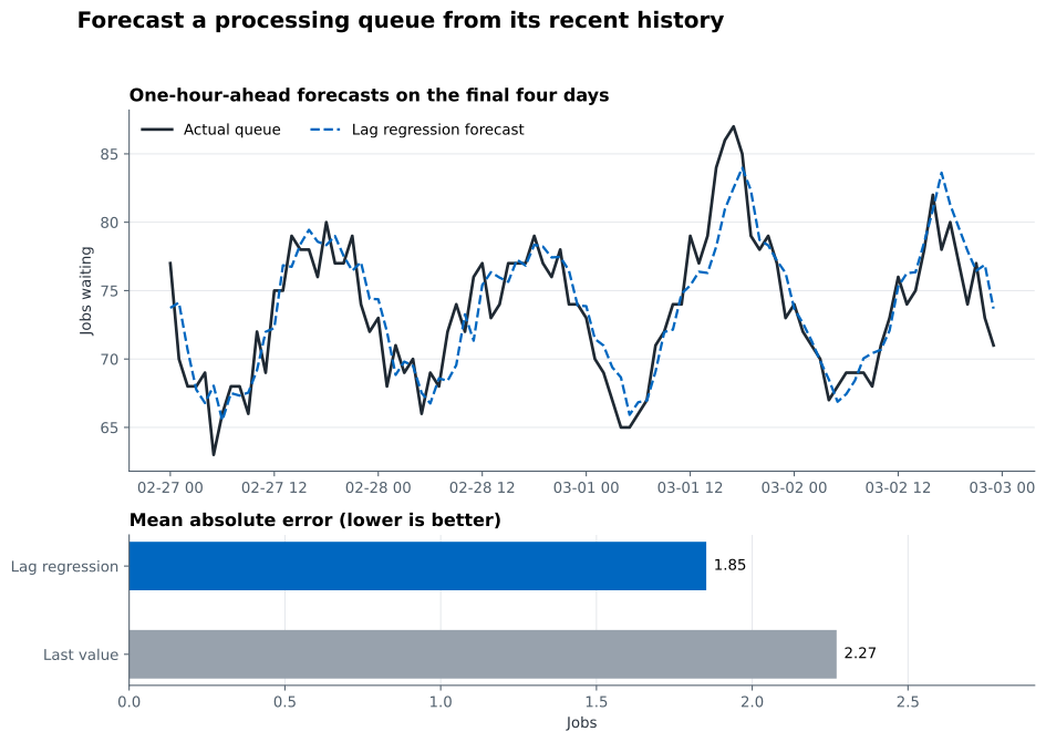
In the upper panel, the dashed forecast follows most rises and falls but smooths some sudden changes. The lower panel confirms that the improvement is not based on one selected hour. Both methods were scored on the same 96 targets.

Refit on all known data and forecast the next hour

After the comparison is complete, fit a fresh model on all 648 usable rows. This uses the test period as known history only after its evaluation role has ended.

Build one new feature row from the latest values. The column names and order must match the training table:

final_model = LinearRegression()
final_model.fit(lagged[feature_names], lagged["jobs_waiting"])

next_timestamp = lagged.index[-1] + pd.Timedelta(hours=1)
next_features = pd.DataFrame(
    [{
        "lag_1": lagged["jobs_waiting"].iloc[-1],
        "lag_2": lagged["jobs_waiting"].iloc[-2],
        "lag_24": lagged["jobs_waiting"].iloc[-24],
    }],
    index=[next_timestamp],
)

next_prediction = final_model.predict(next_features)[0]
print(next_features.to_string())
print(f"\nforecast: {next_prediction:.1f} jobs waiting")

            lag_1  lag_2  lag_24
2025-03-03      71     73      74

forecast: 72.5 jobs waiting

The fitted value is continuous even though the queue is a count. An operations display might round it to 73 jobs, but keep the unrounded value when calculating metrics. The actual count for 3 March is not in the dataset, so this final prediction cannot yet be scored.

In a live process, store the forecast timestamp, inputs, prediction, and later actual value. That record lets you monitor error over time and rebuild the model when queue behavior changes.

Common mistakes and troubleshooting

Using a negative shift. shift(-1) moves a future value onto the current row. That creates leakage. For a next-hour target, features must use positive shifts such as shift(1).

Splitting rows at random. Random training and test rows mix earlier and later periods. Keep a later block for testing, or use a time-series cross-validation plan when comparing settings.

Calling this a four-day-ahead forecast. Test rows after the first hour use actual values observed inside the test period. That is valid for repeated one-hour predictions, not for one prediction made 96 hours in advance.

Ignoring missing timestamps. shift(24) means 24 rows, not automatically 24 elapsed hours. Sort the index, check duplicates, and verify its frequency before treating row lags as time lags.

Choosing many lags before building a baseline. Extra features can fit noise and make coefficients hard to interpret. Start with a few lags suggested by the update interval and repeated patterns, then compare every change on the same later period.

Treating coefficients as causal effects. Past queue values are correlated. A positive coefficient does not prove that one earlier count caused the later count.

Rounding before evaluation. Regression returns decimals. Keep them for scoring so rounding does not hide small improvements. Round only where the final interface requires a whole-job estimate.

Expecting past values to explain new events. A lag-only model cannot know about a new system outage, a policy change, or an incoming batch unless that information appears in the recent queue. Large errors should trigger investigation and may suggest adding known external features.

Recap and next step

An autoregressive forecast converts a series into an ordinary regression table. Each lag column contains a target value that was already known when the new target would be predicted.

The reliable workflow is:

1. Sort the timestamps and verify that the time grid is complete.
2. Create positive lag features that match the forecast horizon.
3. Remove only the early rows that lack enough history.
4. Train on earlier timestamps and test on a later block.
5. Compare the fitted model with a clear baseline on identical rows.
6. Refit on all known data only after evaluation is finished.

For this fictional queue, lags at 1, 2, and 24 hours reduced MAE from 2.27 to 1.85 jobs. The important result is not the exact score. It is the information-safe design: every test prediction uses only values that would have been known before the forecasted hour began.

As a next step, repeat the backtest across several later blocks. If the improvement is stable, test one change at a time, such as a 48-hour lag or a known scheduled-batch feature. Keep the last-value baseline so added complexity always has a fair reference point.