A forecast for Friday can be one day ahead or five days ahead. The date is the same, but the information available to the model is different. A support team that makes its whole staffing plan on Monday cannot use Tuesday’s actual workload to improve Wednesday’s prediction.

To backtest a seven-day time series forecast in Python, choose several historical forecast origins, train only on data before each origin, and predict all seven targets without reading actual values inside that block. Store the origin, target date, and horizon for every prediction, then calculate error separately for days 1 through 7 and compare the same rows with a simple baseline.

We will build that test for a fictional online learning platform. Every Monday, its support team predicts the number of help requests for the next seven days. The lesson uses a transparent linear regression so the evaluation design remains the main subject.

What you need and what the data represents

You need Python 3.11 or newer and a way to run a Python file or notebook cell. You should know basic Python functions and pandas tables. You do not need previous forecasting or regression experience.

Create and activate a virtual environment, then install the four packages used by the executed build:

python -m venv .venv
source .venv/bin/activate
python -m pip install numpy pandas scikit-learn matplotlib

On Windows PowerShell, use .venv\Scripts\Activate.ps1 for the activation step. The executed results use Python 3.13.2, NumPy 2.5.1, pandas 3.0.3, scikit-learn 1.9.0, and Matplotlib 3.11.0.

Download learning_platform_help_requests.csv and save it beside your Python file. It contains 420 consecutive daily counts from 1 January 2024 through 23 February 2025.

This is original synthetic data created with NumPy seed 20260722. Synthetic means code generated the rows. The platform and every count are fictional, and the dataset is released under CC0-1.0 so you may reuse it without restriction. The generation includes a weekly pattern, a gradual rise, a slow cycle, and related day-to-day variation; it does not imitate a real service.

The chart will be saved to a file. Select Matplotlib’s headless Agg backend before importing pyplot so the code also works on servers without a display:

import matplotlib

matplotlib.use("Agg")

import matplotlib.pyplot as plt
import numpy as np
import pandas as pd
from sklearn.linear_model import LinearRegression
from sklearn.metrics import mean_absolute_error

Understanding one origin and seven unavailable targets

A forecast origin is the point in time when a forecast is issued. If the team creates its plan just before Monday begins, that moment is the origin, Sunday is the last day with a known value, and Monday is day 1 of the forecast.

For one origin, the information boundary looks like this:

known history                       hidden from the model
... Fri  Sat  Sun  |  Mon  Tue  Wed  Thu  Fri  Sat  Sun
                   |   1    2    3    4    5    6    7
             forecast origin             horizon days

The forecast horizon is how far a target is from the origin. Monday is one day ahead; Sunday is seven days ahead. The backtest must keep all seven actual values hidden from the model while it creates that forecast block, even though those values are available later for scoring.

This detail separates two tasks:

• A rolling one-day forecast may use Monday’s actual value when predicting Tuesday.
• A fixed seven-day plan cannot use Monday’s actual value because it was unknown when all seven predictions were created.

Our regression uses values from 1, 7, and 14 days earlier. A lag is an earlier observation aligned with the current target row. For later steps, lag 1 is no longer an actual value, so the model must feed its own previous prediction back into the next row. This is a recursive forecast.

The comparison method is seasonal naive forecasting. It predicts each weekday with the count from the same weekday one week earlier. If you want to study that baseline first, see Build and Backtest a Seasonal Naive Forecast in Python.

Load the series and verify the daily timeline

Read the CSV, parse date as a datetime value, sort the rows, and make the dates the index. These checks matter because a seven-row lag represents seven days only when the timeline is complete and ordered.

requests = pd.read_csv(
    "learning_platform_help_requests.csv",
    parse_dates=["date"],
)
requests = requests.set_index("date").sort_index()
series = requests["help_requests"]

print(series.head(8).to_string())
print("\nrows:", len(series))
print("frequency:", pd.infer_freq(series.index))
print("duplicate dates:", series.index.duplicated().sum())
print("missing counts:", series.isna().sum())

The executed output is:

date
2024-01-01     97
2024-01-02     96
2024-01-03     92
2024-01-04     92
2024-01-05     86
2024-01-06     67
2024-01-07     66
2024-01-08    110

rows: 420
frequency: D
duplicate dates: 0
missing counts: 0

D means pandas found one row per calendar day. The counts drop on the first weekend and rise to 110 on the following Monday, so a weekly comparison is reasonable. This preview does not prove that the pattern will remain stable.

If your real file has a missing date, do not treat it as an observed zero. Use a complete daily index to reveal gaps, investigate why they occurred, and define a documented repair rule before creating row-based lags. The current pandas Series.shift() documentation distinguishes shifting values by row from shifting the index with a frequency.

Turn the known history into regression rows

Begin with the first forecast origin immediately before the value at position 336, dated 2 December 2024. The available history ends on 1 December. The function below adds three lag columns and a day_number column, then removes the first 14 rows because they lack enough earlier history.

day_number is known for future dates, so it does not leak a target. It gives the linear model a simple way to represent the gradual change in level.

LAGS = (1, 7, 14)
FIRST_ORIGIN = 336


def make_training_table(history):
    table = pd.DataFrame({"target": history})
    for lag in LAGS:
        table[f"lag_{lag}"] = history.shift(lag)
    table["day_number"] = np.arange(len(table))
    return table.dropna()


history = series.iloc[:FIRST_ORIGIN]
training = make_training_table(history)

print(training.head(5).to_string())
print("\ntraining rows:", len(training))
print("training end:", training.index.max().date())

            target  lag_1  lag_7  lag_14  day_number
date                                                 
2024-01-15     110   64.0  110.0    97.0          14
2024-01-16      99  110.0  110.0    96.0          15
2024-01-17      94   99.0  104.0    92.0          16
2024-01-18      97   94.0   99.0    92.0          17
2024-01-19      92   97.0   89.0    86.0          18

training rows: 322
training end: 2024-12-01

Read the first row from left to right. The target for 15 January is 110 requests. Its lag-1 value is 64 from the previous day, its lag-7 value is 110 from the previous Monday, and its lag-14 value is 97 from two Mondays earlier.

Scikit-learn’s current lagged-feature forecasting example uses the same general conversion from an ordered target to a regression table. It also shows why time-aware evaluation is needed instead of a shuffled split.

Make one complete seven-day forecast

Fit ordinary least-squares linear regression on the 322 available rows. Scikit-learn’s LinearRegression learns an intercept and coefficients that minimize squared training errors.

The next function creates one row at a time. After predicting day 1, it appends that estimate to known_and_predicted. Day 2 therefore receives the day-1 prediction as lag_1, not the hidden actual value.

FORECAST_DAYS = 7
feature_names = ["lag_1", "lag_7", "lag_14", "day_number"]


def recursive_forecast(history, model):
    known_and_predicted = history.astype(float).tolist()
    forecasts = []

    for _ in range(FORECAST_DAYS):
        next_row = pd.DataFrame([{
            "lag_1": known_and_predicted[-1],
            "lag_7": known_and_predicted[-7],
            "lag_14": known_and_predicted[-14],
            "day_number": len(known_and_predicted),
        }])
        next_prediction = float(model.predict(next_row)[0])
        forecasts.append(next_prediction)
        known_and_predicted.append(next_prediction)

    return np.asarray(forecasts)


model = LinearRegression()
model.fit(training[feature_names], training["target"])

recursive = recursive_forecast(history, model)
seasonal = history.iloc[-7:].to_numpy(dtype=float)
actual = series.iloc[FIRST_ORIGIN:FIRST_ORIGIN + 7].to_numpy(dtype=float)

first_forecast = pd.DataFrame({
    "horizon_day": range(1, 8),
    "actual": actual,
    "recursive": recursive,
    "seasonal_naive": seasonal,
}, index=series.index[FIRST_ORIGIN:FIRST_ORIGIN + 7])

print(first_forecast.round(1).to_string())

            horizon_day  actual  recursive  seasonal_naive
date                                                        
2024-12-02            1   137.0      135.7           133.0
2024-12-03            2   130.0      128.7           123.0
2024-12-04            3   127.0      127.5           125.0
2024-12-05            4   119.0      124.3           122.0
2024-12-06            5   112.0      120.2           119.0
2024-12-07            6   100.0      105.6           103.0
2024-12-08            7    94.0      100.1           101.0

The recursive forecast is close on the first three days, then runs high later in the week. This is only one seven-day block. Choosing a method from these seven rows would make the result depend too much on one particular week.

Repeat the test at twelve rolling origins

A rolling-origin backtest repeats the historical simulation at several cutoffs. We move the origin forward seven days each time. The training window expands, but the model never sees a target inside the block it is predicting.

The loop below records the information needed to audit every row. origin_date states when the plan begins, target_date identifies the day being predicted, and horizon_day measures its distance from the origin.

records = []

for origin_position in range(336, len(series) - 7 + 1, 7):
    history = series.iloc[:origin_position]
    training = make_training_table(history)

    model = LinearRegression()
    model.fit(training[feature_names], training["target"])

    recursive = recursive_forecast(history, model)
    seasonal = history.iloc[-7:].to_numpy(dtype=float)
    actual = series.iloc[origin_position:origin_position + 7].to_numpy(dtype=float)
    target_dates = series.index[origin_position:origin_position + 7]

    for horizon, target_date, observed, predicted, baseline in zip(
        range(1, 8), target_dates, actual, recursive, seasonal
    ):
        records.append({
            "origin_date": target_dates[0],
            "target_date": target_date,
            "horizon_day": horizon,
            "actual_requests": int(observed),
            "recursive_regression": predicted,
            "seasonal_naive": baseline,
        })

backtest = pd.DataFrame(records)

print("origins:", backtest["origin_date"].nunique())
print("first origin:", backtest["origin_date"].min().date())
print("last origin:", backtest["origin_date"].max().date())
print("predictions:", len(backtest))

origins: 12
first origin: 2024-12-02
last origin: 2025-02-17
predictions: 84

There are 12 separate, non-overlapping forecast blocks and seven target days in each, giving 84 predictions per method. Their training histories overlap and expand over time. The first plan is made from data through 1 December. The final plan starts on 17 February and covers the dataset’s last seven days.

You can inspect the executed row-level evidence in multi_step_backtest_predictions.csv. This makes it possible to verify any chart point or metric without rerunning the model.

Measure error at each distance

Mean absolute error (MAE) is the average absolute distance between actual and predicted values. It remains in help-request units, and lower is better. The current scikit-learn mean_absolute_error() documentation defines zero as the best possible value.

Calculate MAE separately for each horizon before calculating one overall number:

def horizon_mae(group):
    return pd.Series({
        "recursive_regression": mean_absolute_error(
            group["actual_requests"], group["recursive_regression"]
        ),
        "seasonal_naive": mean_absolute_error(
            group["actual_requests"], group["seasonal_naive"]
        ),
    })


by_horizon = backtest.groupby("horizon_day").apply(
    horizon_mae,
    include_groups=False,
)
overall = pd.Series({
    "recursive_regression": mean_absolute_error(
        backtest["actual_requests"], backtest["recursive_regression"]
    ),
    "seasonal_naive": mean_absolute_error(
        backtest["actual_requests"], backtest["seasonal_naive"]
    ),
})

print(by_horizon.round(2).to_string())
print("\noverall MAE")
print(overall.round(2).to_string())

             recursive_regression  seasonal_naive
horizon_day                                        
1                            5.10            5.00
2                            4.60            5.67
3                            6.01            5.75
4                            5.36            5.67
5                            4.18            4.58
6                            5.58            4.67
7                            4.60            4.67

overall MAE
recursive_regression    5.06
seasonal_naive          5.14

The overall scores are almost tied: recursive regression has an MAE of 5.06 requests, while seasonal naive has an MAE of 5.14. Reporting only those two numbers would hide the useful part of the test.

The regression has lower MAE on horizons 2, 4, 5, and 7. The seasonal baseline has lower MAE on horizons 1, 3, and 6. Neither method wins at every distance, and this synthetic example does not establish that the 0.08-request overall gap will generalize to other data.

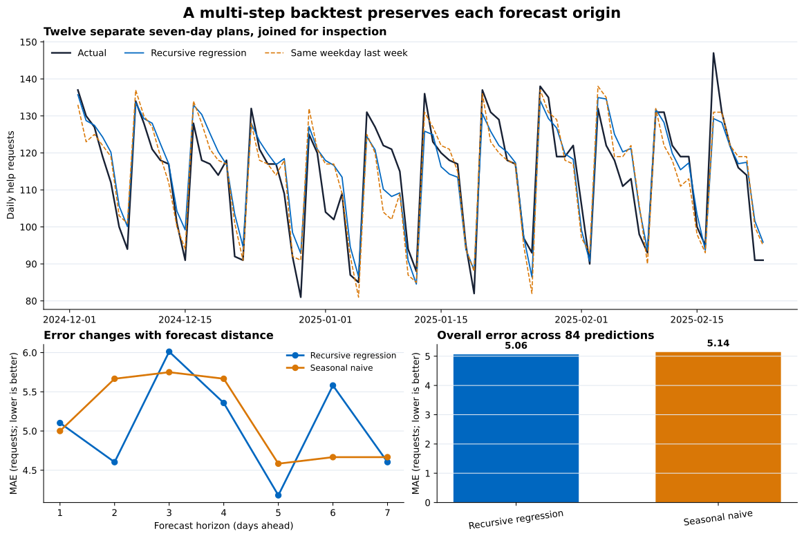
Read the lower-left panel before the overall bars. It shows where each method makes its errors. Then use the upper timeline to check whether misses cluster in a particular week instead of trusting one average.

Common mistakes that change the question being tested

Using actual values from inside the seven-day block. If Tuesday’s actual becomes Wednesday’s lag 1, the code is testing repeated one-day forecasts. For a Monday plan, append Tuesday’s prediction instead.

Fitting once on all 420 rows. That lets later targets influence coefficients used at earlier origins. Refit at each origin using only series.iloc[:origin_position].

Shuffling train and test rows. Random splitting breaks the direction of time and may place later observations in training. Keep the order and simulate the real update schedule.

Scoring only one origin. One unusual week can favor either model. Use several origins that cover the operating conditions you expect, and keep a later untouched period if you also tune features or model settings.

Averaging every horizon immediately. An overall MAE can hide a method that is reliable tomorrow but weak one week ahead. Preserve horizon_day and report the distances that matter to the decision.

Overlapping origins without noticing repeated targets. Moving the origin one day at a time for seven-day forecasts makes a target appear in several test blocks. That can be valid, but predictions are then related and some dates receive more weight. This lesson steps forward seven days so each target appears once.

Treating seven rows as seven days without checking dates. Duplicate or missing dates break the meaning of row lags. Validate the time index before feature creation.

Calling the small MAE difference a general model victory. These results belong to one synthetic series and 12 origins. Compare uncertainty across origins, operational costs, and performance on current real data before choosing a production method.

Assuming recursion is the only multi-step strategy. A direct strategy fits a separate model for each horizon. A multi-output model predicts all horizons together. Each strategy needs the same origin-safe evaluation, but its training table and error behavior differ.

Recap: a checklist for your next forecast

Multi-step forecasting is mainly an information-timing problem. Write down when the forecast is created, how many future values are produced together, and when actual values become available. Those facts determine which inputs are legal.

For a trustworthy backtest:

1. Verify that timestamps are ordered, unique, and regularly spaced.
2. Define the forecast origin, horizon, and update schedule in plain language.
3. Hide the complete future block at every historical origin.
4. Recreate later inputs from predictions when actual values would be unknown.
5. Record origin, target date, and horizon with every prediction.
6. Compare the same targets with a simple baseline.
7. Report error by horizon before reducing it to one overall score.

Here, twelve seven-day plans produced 84 predictions for each method. Recursive regression reached 5.06 requests MAE and seasonal naive reached 5.14, but their horizon-level wins were mixed. The durable result is the backtest design, not the small difference between those scores.

Next, group the row-level absolute errors by origin_date. That view will show whether one difficult week controls the average. If you then change the lag set or compare a direct model, reserve a final block of origins that those choices never see.