Calculate Bayes Theorem from a Frequency Table in Python

A greenhouse moisture sensor sends an alert when soil may be too dry. The sensor catches many dry-soil cases, but it also sends some false alerts. When an alert arrives, what is the probability that the soil is actually dry?

The sensor’s alert rate on dry soil is not enough to answer that question. You also need to know how often the soil is dry before any alert arrives and how often the sensor produces a false alert. Bayes theorem combines those pieces of information.

In this tutorial, you will calculate Bayes theorem from a small frequency table, implement the same calculation as a Python function, and verify the result by counting rows with pandas. You will then change the starting dry-soil rate to see why the same alert can mean different things in different settings.

Prerequisites and setup

You need Python 3.11 or later and basic experience with variables and functions. You do not need previous knowledge of probability or pandas tables.

Create a virtual environment and install the packages used in the lesson:

python -m venv .venv
source .venv/bin/activate
python -m pip install pandas numpy matplotlib

On Windows PowerShell, activate the environment with .venv\Scripts\Activate.ps1. The published results were executed with Python 3.13.2, pandas 3.0.3, NumPy 2.5.1, and Matplotlib 3.11.0.

Download the tutorial’s greenhouse_sensor_readings.csv file. It is an original synthetic dataset released under CC0-1.0. The 1,000 fictional readings were designed for teaching and do not describe a real greenhouse or sensor.

Place the CSV in the same folder as your Python file or notebook. Then load it and inspect five rows:

import pandas as pd

readings = pd.read_csv("greenhouse_sensor_readings.csv")
print(readings.head().to_string(index=False))
print("shape:", readings.shape)

reading_id soil_condition sensor_result
   GH-0001         not dry         alert
   GH-0002         not dry      no alert
   GH-0003         not dry      no alert
   GH-0004         not dry      no alert
   GH-0005         not dry      no alert
shape: (1000, 3)

Each row represents one sensor reading and its corresponding reference soil check. sensor_result is what the automated sensor reported. soil_condition is the condition found by the reference check. For this lesson, that check provides the known soil condition against which the sensor result is compared.

Mental model: start with counts you can inspect

Bayes theorem is easier to understand when you can see every group in a table. A frequency table counts how often combinations of categories occur. Here, the rows describe the real soil condition and the columns describe the sensor result.

The next code uses pd.crosstab to build that table. margins=True adds totals. The pandas crosstab documentation defines the default result as a frequency table when no values or aggregation function are supplied.

frequency = pd.crosstab(
    readings["soil_condition"],
    readings["sensor_result"],
    margins=True,
)

frequency = frequency.reindex(
    index=["dry", "not dry", "All"],
    columns=["alert", "no alert", "All"],
)
print(frequency)

sensor_result   alert  no alert   All
soil_condition
dry               150        50   200
not dry            80       720   800
All               230       770  1000

Read one direction at a time. Of the 200 dry-soil readings, 150 produced an alert. Of the 800 readings that were not dry, 80 still produced an alert. Those 80 are false alerts.

Now read down the alert column. There were 230 alerts in total: 150 when the soil was dry and 80 when it was not dry. This column already contains the answer to our question. Among the 230 alerts, 150 came from dry soil:

dry_given_alert_by_count = 150 / 230
print(f"P(dry | alert) by counting: {dry_given_alert_by_count:.1%}")

P(dry | alert) by counting: 65.2%

The vertical bar in P(dry | alert) means given. The expression asks for the probability of dry soil given that an alert occurred. It does not ask for the probability of an alert given dry soil. Direction matters.

Map the greenhouse question to Bayes theorem

A conditional probability is the probability of one event when another event is known. Bayes theorem relates conditional probabilities in opposite directions. We know how often the sensor alerts under each soil condition, but we want the probability of the soil condition after observing an alert.

For this problem, the formula is:

P(dry | alert) = P(alert | dry) × P(dry) / P(alert)

The four quantities have common names:

• The prior, P(dry), is the dry-soil probability before seeing the current sensor result.
• The likelihood for the observed alert, P(alert | dry), is the probability of that alert when the soil is dry.
• The evidence, P(alert), is the overall probability of receiving an alert.
• The posterior, P(dry | alert), is the updated dry-soil probability after an alert.

Calculate the first two values from the table:

prior = frequency.loc["dry", "All"] / frequency.loc["All", "All"]
alert_if_dry = frequency.loc["dry", "alert"] / frequency.loc["dry", "All"]

print(f"prior P(dry): {prior:.1%}")
print(f"likelihood P(alert | dry): {alert_if_dry:.1%}")

prior P(dry): 20.0%
likelihood P(alert | dry): 75.0%

The prior is 20% because 200 of 1,000 readings had dry soil. The likelihood is 75% because the sensor alerted for 150 of those 200 dry readings.

Do not reverse the likelihood. P(alert | dry) is 75%, but P(dry | alert) is 65.2%. The two probabilities use different denominators: 200 dry readings for the first and 230 alerts for the second.

Calculate the missing evidence

The overall alert probability can be counted directly as 230 / 1000. In a new setting, however, you may only know the prior and the sensor’s behavior. You can calculate the evidence by considering both routes to an alert:

P(alert) = P(alert | dry) × P(dry)
         + P(alert | not dry) × P(not dry)

The first route is a correct alert on dry soil. The second is a false alert on soil that is not dry. Calculate the false-alert rate and combine both routes:

alert_if_not_dry = (
    frequency.loc["not dry", "alert"]
    / frequency.loc["not dry", "All"]
)
not_dry_prior = 1 - prior

alert_probability = (
    alert_if_dry * prior
    + alert_if_not_dry * not_dry_prior
)

print(f"P(alert | not dry): {alert_if_not_dry:.1%}")
print(f"P(alert): {alert_probability:.1%}")

P(alert | not dry): 10.0%
P(alert): 23.0%

The two routes contribute 0.75 × 0.20 = 0.15 and 0.10 × 0.80 = 0.08. Together they give 0.23, or 23%. This agrees with the table: 230 of 1,000 readings produced an alert.

Now substitute the values into Bayes theorem:

posterior = alert_if_dry * prior / alert_probability
print(f"P(dry | alert): {posterior:.1%}")

P(dry | alert): 65.2%

An alert raises the dry-soil probability from 20% to about 65.2%. That is useful evidence, but it is not certainty. About 34.8% of alerts in this designed dataset occur when the soil is not dry.

Put the calculation in a reusable function

A function makes the calculation explicit and lets you test other situations. It accepts the prior, the alert rate when dry, and the false-alert rate when not dry:

def bayes_probability(prior, alert_if_dry, alert_if_not_dry):
    alert_probability = (
        alert_if_dry * prior
        + alert_if_not_dry * (1 - prior)
    )
    return alert_if_dry * prior / alert_probability


result = bayes_probability(
    prior=0.20,
    alert_if_dry=0.75,
    alert_if_not_dry=0.10,
)
print(f"posterior from function: {result:.4f}")

posterior from function: 0.6522

Verify the formula against the table instead of trusting one implementation:

counted_result = (
    frequency.loc["dry", "alert"]
    / frequency.loc["All", "alert"]
)

print(f"formula: {result:.6f}")
print(f"counting: {counted_result:.6f}")
print("match:", abs(result - counted_result) < 1e-12)

formula: 0.652174
counting: 0.652174
match: True

This agreement is a practical test of the code. Direct counting works when you have a representative labeled table. The formula is valuable when you know the rates but do not have all individual rows in one dataset.

See how the prior changes the answer

Suppose the same sensor keeps its 75% alert rate on dry soil and 10% false-alert rate. Its alert does not have one universal meaning. The posterior also depends on the prior dry-soil rate.

Use the function with three starting rates:

for prior_dry_rate in [0.05, 0.20, 0.40]:
    updated = bayes_probability(
        prior_dry_rate,
        alert_if_dry=0.75,
        alert_if_not_dry=0.10,
    )
    print(
        f"prior {prior_dry_rate:>5.0%} -> "
        f"posterior {updated:>5.1%}"
    )

prior    5% -> posterior 28.3%
prior   20% -> posterior 65.2%
prior   40% -> posterior 83.3%

When dry soil is rare at 5%, most alerts still come from the much larger not-dry group. The alert raises the probability, but only to 28.3%. When the prior is 40%, the same sensor alert raises the posterior to 83.3%.

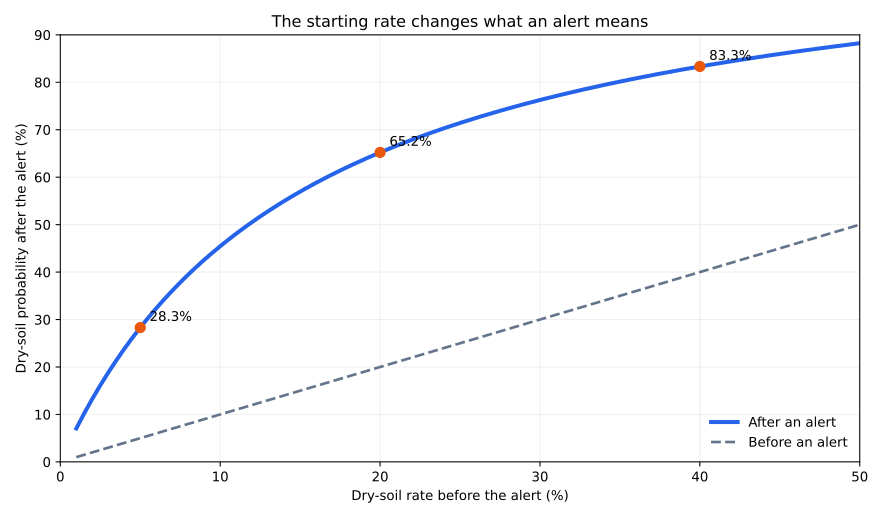
Read the horizontal axis as the probability before an alert and the blue curve as the updated probability. The dashed diagonal shows no change. The blue curve stays above it because this sensor alerts more often for dry soil than for soil that is not dry. The gap is not constant, which is why you should calculate the update rather than add a fixed number of percentage points.

This is the durable lesson behind base rates. A base rate is the starting frequency of an event. If the greenhouse enters a rainy season, changes its irrigation schedule, or applies the sensor to a different growing area, the dry-soil prior may change. Reusing an old posterior without updating the prior can mislead a decision.

Common mistakes and troubleshooting

Reversing the condition. P(alert | dry) and P(dry | alert) answer different questions. Write each denominator in words: “among dry readings” versus “among alerts.” A frequency table makes the difference visible.

Ignoring false alerts. The likelihood for dry soil is only one route to an alert. The evidence must also include P(alert | not dry) × P(not dry). Leaving out this route makes the posterior incorrectly equal to 100%.

Using percentages as whole numbers. Python expects 0.20 for 20%, not 20. Keep all inputs on the zero-to-one scale, then use a format such as .1% when displaying them.

Using a prior from the wrong setting. A prior estimated in one season, location, or operating policy may not fit another. Record where the starting rate came from and check whether conditions changed.

Treating synthetic results as sensor specifications. The 75% and 10% rates were designed for this lesson. Estimate rates from appropriate validation data before applying the workflow to a real system. The measurements should represent the population where the calculation will be used.

Dividing by zero. If both routes to an alert have zero probability, then P(alert) is zero and the conditional probability after an alert is undefined. Validate that inputs are between zero and one and that the calculated evidence is greater than zero.

Combining dependent signals as if they were independent. This tutorial updates on one alert. Multiplying likelihoods for several sensor readings requires additional assumptions about how those readings depend on one another. Do not treat repeated readings from the same device as independent without checking the data-generating process.

Recap

Bayes theorem updates a starting probability with observed evidence. In the greenhouse example, the prior dry-soil rate was 20%, the sensor alerted for 75% of dry readings, and it falsely alerted for 10% of not-dry readings. Those values produced a 23% overall alert rate and a 65.2% posterior probability of dry soil after an alert.

The practical workflow is to build an inspectable frequency table, keep the direction of each conditional probability clear, include every route to the evidence, calculate the posterior, and verify it by direct counting when labeled data is available. Most importantly, reconsider the prior when the setting changes.

If you want to continue from probability updates to a model that combines word evidence across several categories, see routing support tickets with Naive Bayes in Python.