Large hosted text generators can make language models seem mysterious. A much smaller model makes the central prediction task visible: given the text so far, which token should come next?

To build a bigram language model in Python, split training sentences into tokens, count every adjacent token pair, and divide each pair count by all counts that share the same first token. Use those probabilities to sample text, add smoothing when scoring unseen pairs, and calculate perplexity on a separate test set.

This tutorial builds that complete process from simple word-pair counts. The model will learn from fictional equipment-repair notes. It is intentionally small: it cannot understand meaning or remember a full sentence, but you can inspect every result.

Before You Begin: Setup and Data

You need Python 3.10 or later and basic knowledge of lists, dictionaries, and functions. The lesson uses pandas to read a table, NumPy to make repeatable weighted samples, and Matplotlib to create a chart.

Create a virtual environment and install the packages. On macOS or Linux, run:

python -m venv .venv
source .venv/bin/activate
python -m pip install numpy pandas matplotlib

On Windows PowerShell, run python -m venv .venv, activate it with .venv\Scripts\Activate.ps1, and then run the same pip install command.

The executed build used Python 3.13.2, NumPy 2.5.1, pandas 3.0.3, and Matplotlib 3.11.0. Download the synthetic repair-note dataset and save it as repair_notes.csv beside your Python file.

The dataset contains 44 short notes: 36 training rows and 8 test rows. It was created for this lesson and is released under CC0 1.0. All note IDs, equipment states, and messages are fictional. The test rows combine known words in new ways. This design lets us check how the model handles word pairs that did not appear during training.

Load the table and inspect a few rows before building the model:

import pandas as pd

notes = pd.read_csv("repair_notes.csv")
train_notes = notes.loc[notes["split"].eq("train"), "text"]
test_notes = notes.loc[notes["split"].eq("test"), "text"]

print(f"rows: {len(notes)} (train={len(train_notes)}, test={len(test_notes)})")
print(notes.head().to_string(index=False))

The real output is:

rows: 44 (train=36, test=8)
note_id split                         text
   R001 train      printer needs new paper
   R002 train      printer needs new toner
   R003 train             printer is ready
   R004 train           printer is offline
   R005 train scanner needs quick cleaning

The split column identifies which notes belong to each group. The model learns only from train rows, and we keep the test rows separate until evaluation so they cannot influence the counts.

How a Bigram Language Model Works

A token is one unit of text. Our tokenizer extracts alphabetic words and converts them to lowercase, so Printer needs paper. becomes three tokens: printer, needs, and paper.

A bigram is a pair of adjacent tokens. That sentence contains these pairs:

<s> -> printer
printer -> needs
needs -> paper
paper -> </s>

<s> and </s> are boundary markers. They teach the model which words can begin or end a note. They are model symbols, not words that appear in the CSV.

The bigram assumption is strict: the next-token probability depends only on the current token. For example, the model estimates:

P(new | needs) = count(needs -> new) / count(all pairs starting with needs)

It does not remember whether the note began with printer or sensor. This limited memory makes the model easy to study, but it also explains why generated text may combine equipment and repairs in unusual ways.

Modern next-token systems use much richer context. After this count-based foundation, causal self-attention in NumPy shows one mechanism that lets a model use several earlier tokens while blocking later ones.

Count Training Pairs in Python

First, define the tokenizer. The regular expression keeps runs of letters and converts the text to lowercase. This policy is suitable for the simple English notes, but a production tokenizer must define how to handle numbers, punctuation, other writing systems, and parts of words.

import re

def tokenize(text):
    return re.findall(r"[a-z]+", text.lower())

print(tokenize("Printer needs new paper."))

['printer', 'needs', 'new', 'paper']

Now count the pairs. A Counter stores each item as a key and its count as the corresponding value. The Python documentation for collections.Counter describes it as a dictionary subclass for counting hashable objects.

from collections import Counter, defaultdict

START = "<s>"
END = "</s>"

def build_counts(texts):
    next_counts = defaultdict(Counter)
    vocabulary = set()

    for text in texts:
        words = tokenize(text)
        vocabulary.update(words)
        sequence = [START, *words, END]

        for current_token, next_token in zip(sequence, sequence[1:]):
            next_counts[current_token][next_token] += 1

    return next_counts, sorted(vocabulary)

next_counts, vocabulary = build_counts(train_notes)

print("vocabulary size:", len(vocabulary))
print(next_counts["needs"].most_common())

The executed result is:

vocabulary size: 32
[('new', 6), ('quick', 5), ('careful', 4)]

There are 32 ordinary words in the training vocabulary. After needs, the training data contains new six times, quick five times, and careful four times. The total number of observed continuations after needs is therefore 15.

Turn Counts into Next-Token Probabilities

Raw relative frequency assigns new a probability of 6 / 15 = 0.4. It assigns zero to every unseen pair, including needs -> ready.

Zero creates a problem during evaluation. If one pair in a test note has probability zero, the product of all pair probabilities for that note is zero. Add-one smoothing avoids that result by adding one imaginary count to every possible next token:

smoothed probability =
    (observed pair count + 1)
    / (all counts after current token + number of choices)

The next function uses alpha for the count added to every choice. Set alpha=1.0 for add-one smoothing, a smaller value such as 0.1 for lighter smoothing, or 0.0 for no smoothing.

def next_probability(
    current_token,
    next_token,
    next_counts,
    vocabulary,
    alpha=1.0,
):
    choices = [*vocabulary, END]
    if next_token not in choices:
        return 0.0

    observed = next_counts[current_token][next_token]
    total = sum(next_counts[current_token].values())

    return (
        (observed + alpha)
        / (total + alpha * len(choices))
    )

Print four selected probabilities to see what smoothing changes:

for token in ("new", "quick", "careful", "ready"):
    probability = next_probability(
        "needs", token, next_counts, vocabulary, alpha=1.0
    )
    print(f"P({token:>7} | needs) = {probability:.3f}")

P(    new | needs) = 0.146
P(  quick | needs) = 0.125
P(careful | needs) = 0.104
P(  ready | needs) = 0.021

new remains the most likely of these tokens because it has the largest observed count. The three observed continuations have lower probabilities after smoothing because probability mass is now shared across 33 choices: 32 words plus </s>. In contrast, ready rises from zero to 0.021 even though it never appeared after needs.

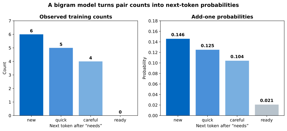
Read the left panel as evidence from the training rows. The right panel shows the corresponding values from the model’s smoothed distribution. The small bar for ready is not new evidence; it is probability assigned to an unseen pair by the smoothing rule.

Generate a Note One Token at a Time

Text generation repeats one operation: calculate a distribution after the current token, sample one next token, and use that sample as the new current token. Generation stops when it samples </s> or reaches a safety limit.

For this demonstration, use only observed transitions by setting alpha=0.0. This keeps the tiny corpus from assigning probability to many unseen paths. NumPy’s Generator.choice documentation accepts a probability vector through p. The NumPy random sampling guide recommends creating a dedicated generator with default_rng.

import numpy as np

def generate_note(
    next_counts,
    vocabulary,
    rng,
    alpha=0.0,
    max_words=8,
):
    choices = np.array([*vocabulary, END], dtype=object)
    current_token = START
    output = []

    for _ in range(max_words):
        probabilities = np.array([
            next_probability(
                current_token,
                candidate,
                next_counts,
                vocabulary,
                alpha,
            )
            for candidate in choices
        ])
        probabilities /= probabilities.sum()
        next_token = str(rng.choice(choices, p=probabilities))

        if next_token == END:
            break

        output.append(next_token)
        current_token = next_token

    return " ".join(output)

Create one generator with a fixed seed, then reuse it for five samples:

rng = np.random.default_rng(20260727)

for index in range(1, 6):
    print(
        f"{index}. "
        f"{generate_note(next_counts, vocabulary, rng)}"
    )

The executed samples are:

1. camera reports weak signal
2. projector needs new toner
3. router is ready
4. camera needs new toner
5. printer is stable

Every adjacent pair in these notes appeared during training, although some complete notes did not. For example, projector -> needs, needs -> new, and new -> toner are known pairs, so the model can join them into projector needs new toner.

This result also shows the limitation. The model cannot check whether toner belongs to a projector because it remembers only one token. A fixed seed makes this lesson’s output repeatable, but it does not make the samples uniquely correct. A different seed can produce different valid samples from the same distribution.

Test the Model with Perplexity

Generation shows what the model can sample. Evaluation asks how much probability the model assigns to notes kept outside training.

Perplexity summarizes the model’s average surprise across all evaluated pairs. Lower is better when models use the same tokenization, vocabulary, and test data. A perplexity of 5 can be read loosely as uncertainty similar to choosing among five equally likely next tokens at each step. Perplexity is not accuracy, and values from unrelated datasets are usually not comparable.

The function below adds the negative logarithm of each pair probability, divides by the number of pairs, and converts the result back from the logarithmic scale. Logarithms prevent a product of many small probabilities from becoming too small for normal floating-point arithmetic.

import math

def perplexity(
    texts,
    next_counts,
    vocabulary,
    alpha,
):
    negative_log_sum = 0.0
    pair_count = 0

    for text in texts:
        sequence = [START, *tokenize(text), END]

        for current_token, next_token in zip(
            sequence, sequence[1:]
        ):
            probability = next_probability(
                current_token,
                next_token,
                next_counts,
                vocabulary,
                alpha,
            )
            if probability == 0:
                return math.inf

            negative_log_sum -= math.log(probability)
            pair_count += 1

    return math.exp(negative_log_sum / pair_count)

Compare no smoothing, a small smoothing value, and add-one smoothing on the same eight test rows:

print(
    "train perplexity (alpha=1.0):",
    f"{perplexity(train_notes, next_counts, vocabulary, 1.0):.2f}",
)
print(
    "test perplexity  (alpha=0.0):",
    perplexity(test_notes, next_counts, vocabulary, 0.0),
)
print(
    "test perplexity  (alpha=0.1):",
    f"{perplexity(test_notes, next_counts, vocabulary, 0.1):.2f}",
)
print(
    "test perplexity  (alpha=1.0):",
    f"{perplexity(test_notes, next_counts, vocabulary, 1.0):.2f}",
)

train perplexity (alpha=1.0): 11.23
test perplexity  (alpha=0.0): inf
test perplexity  (alpha=0.1): 4.63
test perplexity  (alpha=1.0): 11.89

The unsmoothed test result is infinite because at least one test pair was unseen. Additive smoothing gives every in-vocabulary pair a nonzero probability. On this small synthetic test set, alpha=0.1 produces lower perplexity than alpha=1.0; adding a full count spreads more probability across unseen choices and leaves less for observed pairs.

Do not select alpha on the final test set in a real experiment. Use a third validation set to choose it, then report the test result once. Also do not conclude that 0.1 is a universal setting. Its usefulness depends on the corpus size and vocabulary.

Common Mistakes and Troubleshooting

The model reports a zero probability or infinite perplexity. An unseen pair received no probability. Use smoothing for evaluation, and confirm that each word belongs to the training vocabulary. A real system often maps unknown words to a special <unk> token; this small dataset avoids unknown test words so we can focus on unseen pairs.

Probabilities do not sum to one. Use the same set of possible next tokens in every numerator and denominator. Include </s> because ending a note is a possible next event. Do not include <s> as a next token.

Generation never stops. Add </s> to every training sequence and keep max_words as a safety limit. Without an end marker, the model has no learned way to finish.

The same seed gives unexpected text after a code change. A seed reproduces the sequence of random draws only when the candidate order, probabilities, package behavior, and number of earlier draws remain the same. Sort the vocabulary, as this tutorial does, and record package versions with important experiments.

Test perplexity looks better than training perplexity. That can happen here because smoothing strongly penalizes the training distribution while the tiny test set contains many common patterns. Perplexity is an average over different pairs. Use larger representative splits before drawing a performance conclusion.

Generated text is grammatical but factually strange. That is expected from one-token memory. A bigram model learns local pair frequency, not equipment rules, meaning, or truth. Improve the data and evaluation first; then consider longer n-grams or models that use a wider context.

Recap: What the Counts Teach

A bigram language model is a next-token table built from adjacent pairs. Counting provides the evidence, normalization turns counts into probabilities, boundary markers teach starts and stops, and weighted sampling turns the table back into text.

The separate test split exposed the model’s most important weakness: seeing every word during training does not mean the model has seen every pair. Smoothing prevents one unseen pair from making the probability of a complete note zero, while perplexity summarizes the remaining probability assignments on one fixed test set.

This model is not a smaller substitute for a modern large language model. Its value is clarity. You can inspect every count, reproduce every output, and see exactly where short context helps and where it fails.