How to Calculate Bayes Error for Gaussian Classes in Python

A classifier reaches 83.9% accuracy on a clean test set. Is the missing 16.1% caused by a weak model, or do the classes overlap so much that the available measurement cannot prevent every mistake?

To calculate Bayes error for Gaussian classes, multiply each class’s Gaussian density by its prior probability, choose the larger value at every possible measurement, and integrate the smaller value with numpy.trapezoid. That overlap area is the lowest expected classification error for the stated distributions, priors, features, and equal mistake costs.

This tutorial makes that limit visible with one numeric feature. Two fictional production lines apply coating to sheets. We know how each line’s measurement is distributed, so we can calculate the best theoretical rule before fitting a model. We will then check a learned Gaussian Naive Bayes classifier on data it did not see during training.

Setup, prerequisites, and synthetic data

You need Python 3.11 or newer. You should be comfortable with Python functions and pandas tables. You do not need previous knowledge of calculus or Bayesian classification; the small amount of numerical integration is explained when it appears.

Create a virtual environment and install the packages used in the executed lesson:

python -m venv .venv
source .venv/bin/activate
python -m pip install numpy pandas scikit-learn matplotlib

On Windows PowerShell, activate the environment with .venv\Scripts\Activate.ps1. The results below were executed with Python 3.13.2, NumPy 2.5.1, pandas 3.0.3, scikit-learn 1.9.0, and Matplotlib 3.11.0.

Download coating_measurements.csv and save it in the same directory as your Python file or notebook. The 4,000 rows are original synthetic teaching data released under CC0-1.0. The sheet identifiers, production lines, and coating values are fictional and do not describe a real factory or process.

The reproducible generator uses a fixed random seed and these known population settings:

• Line A produces 65% of the sheets. Its coating measurement has mean 48 g/m² and standard deviation 5.5 g/m².
• Line B produces 35% of the sheets. Its coating measurement has mean 58 g/m² and standard deviation 5.5 g/m².

A mean is the center of a numeric distribution. A standard deviation describes its typical spread around that center. The two means are different, but both distributions have tails that occupy some of the same measurement range.

Select Matplotlib’s non-interactive Agg backend before importing pyplot. This allows the executed build to save an SVG without opening a desktop window. Then load the CSV and inspect five rows:

import matplotlib

matplotlib.use("Agg")

import matplotlib.pyplot as plt
import numpy as np
import pandas as pd

measurements = pd.read_csv("coating_measurements.csv")
print(measurements.head().to_string(index=False))
print("shape:", measurements.shape)

sheet_id production_line  coating_g_m2 split
 CS-0001          line_A        53.169  test
 CS-0002          line_B        62.720 train
 CS-0003          line_A        52.011 train
 CS-0004          line_A        45.176 train
 CS-0005          line_A        45.360 train
shape: (4000, 4)

Each row contains one coating measurement and its known production line. The split column reserves 3,000 rows for learning and 1,000 rows for one final check. We will not use the test labels to estimate the model.

How weighted Gaussian evidence works

A classifier maps an input to a class. Here, the input is one coating measurement, and the classes are line_A and line_B.

A Gaussian distribution is the familiar symmetric bell-shaped curve. Its probability density describes where numeric values are concentrated. Density is not the probability of one exact continuous value. Instead, an area under the curve across a range represents probability.

For a measurement x, the Gaussian density for each line is its likelihood: how compatible that measurement is with the line. The prior is the class probability before seeing x. Multiply them to get an unnormalized joint score:

line score = P(line) × density(x | line)

The Bayes decision chooses the line with the larger score. Dividing both scores by their sum would turn them into posterior probabilities, but that common denominator cannot change which score is larger.

The prior matters. Line A is more common, so a borderline sheet needs somewhat stronger evidence before the rule changes to line B. The boundary will therefore not sit exactly halfway between the means.

First, store the known parameters. The function below implements the Gaussian density directly so every part of the calculation remains visible:

class_parameters = {
    "line_A": {"prior": 0.65, "mean": 48.0, "std": 5.5},
    "line_B": {"prior": 0.35, "mean": 58.0, "std": 5.5},
}

def gaussian_pdf(values, mean, std):
    exponent = -0.5 * ((values - mean) / std) ** 2
    return np.exp(exponent) / (std * np.sqrt(2 * np.pi))

def joint_scores(values):
    line_a = class_parameters["line_A"]
    line_b = class_parameters["line_B"]
    score_a = line_a["prior"] * gaussian_pdf(
        values, line_a["mean"], line_a["std"]
    )
    score_b = line_b["prior"] * gaussian_pdf(
        values, line_b["mean"], line_b["std"]
    )
    return score_a, score_b

The term pdf means probability density function. The formula returns one density height for every value in a NumPy array. Multiplying by the class prior makes the two curves comparable for a decision.

Inspect three decisions before integrating

Before calculating an area, check individual measurements that can be understood by eye. We will compare 50, 55, and 60 g/m². Normalizing the two scores makes the result easier to read as posterior probabilities:

def bayes_predictions(values):
    score_a, score_b = joint_scores(values)
    return np.where(score_b > score_a, "line_B", "line_A")

example_values = np.array([50.0, 55.0, 60.0])
example_a, example_b = joint_scores(example_values)
example_total = example_a + example_b

example_table = pd.DataFrame({
    "coating_g_m2": example_values,
    "P(line_A | x)": example_a / example_total,
    "P(line_B | x)": example_b / example_total,
    "decision": bayes_predictions(example_values),
})
print(example_table.round(3).to_string(index=False))

 coating_g_m2  P(line_A | x)  P(line_B | x) decision
         50.0          0.834          0.166   line_A
         55.0          0.489          0.511   line_B
         60.0          0.155          0.845   line_B

At 50 g/m², line A has about 83.4% of the posterior probability. At 60 g/m², line B has about 84.5%. The 55 g/m² case is close, but line B’s score is slightly larger, so the rule chooses line B.

These probabilities are correct for the designed distributions and priors. They are not confidence ratings that can be transferred to real coating data.

Find the boundary and integrate Bayes error

The decision boundary is the measurement where the two weighted densities are equal. Values on one side choose line A; values on the other side choose line B.

Create a dense ordered grid, calculate both scores, and find where their comparison changes. Taking the midpoint of the two grid positions gives a numerical boundary:

grid = np.linspace(10.0, 95.0, 100_001)
score_a, score_b = joint_scores(grid)

changes = np.flatnonzero(
    np.diff((score_b > score_a).astype(int))
)
boundary = (grid[changes[0]] + grid[changes[0] + 1]) / 2
print(f"decision boundary: {boundary:.2f} g/m²")

decision boundary: 54.87 g/m²

The midpoint between the two means is 53 g/m², but the best boundary is farther toward line B’s mean. This gives the more common line A a wider decision region. If the priors were equal and the standard deviations remained equal, the boundary would return to the midpoint.

Why does the smaller curve represent error? At any measurement, the rule selects the class with the larger weighted density. Cases that came from the other class are mistakes, and their local probability is the smaller weighted density.

NumPy’s trapezoid function approximates an integral by adding thin trapezoid areas along an ordered grid. Integrate the smaller score at every grid point, then subtract that error from 1 to get the best expected accuracy:

bayes_error = np.trapezoid(
    np.minimum(score_a, score_b),
    x=grid,
)
bayes_accuracy = 1 - bayes_error

choose_line_b = score_b > score_a
line_a_misclassification = np.trapezoid(
    np.where(choose_line_b, score_a, 0.0), x=grid
)
line_b_misclassification = np.trapezoid(
    np.where(~choose_line_b, score_b, 0.0), x=grid
)

print(f"Bayes error: {bayes_error:.4f}")
print(f"Bayes accuracy limit: {bayes_accuracy:.4f}")
print(f"line_A misclassification contribution: {line_a_misclassification:.4f}")
print(f"line_B misclassification contribution: {line_b_misclassification:.4f}")

Bayes error: 0.1684
Bayes accuracy limit: 0.8316
line_A misclassification contribution: 0.0687
line_B misclassification contribution: 0.0997

The two contributions add to 0.1684, or 16.84%. About 6.87 percentage points come from line A sheets that fall in the line B decision region. About 9.97 points come from line B sheets that fall in line A’s region.

The resulting 83.16% accuracy is an expected long-run limit under four fixed conditions: these Gaussian distributions, these priors, this single feature, and equal cost for either kind of mistake. It is not a universal limit for every possible dataset or feature set.

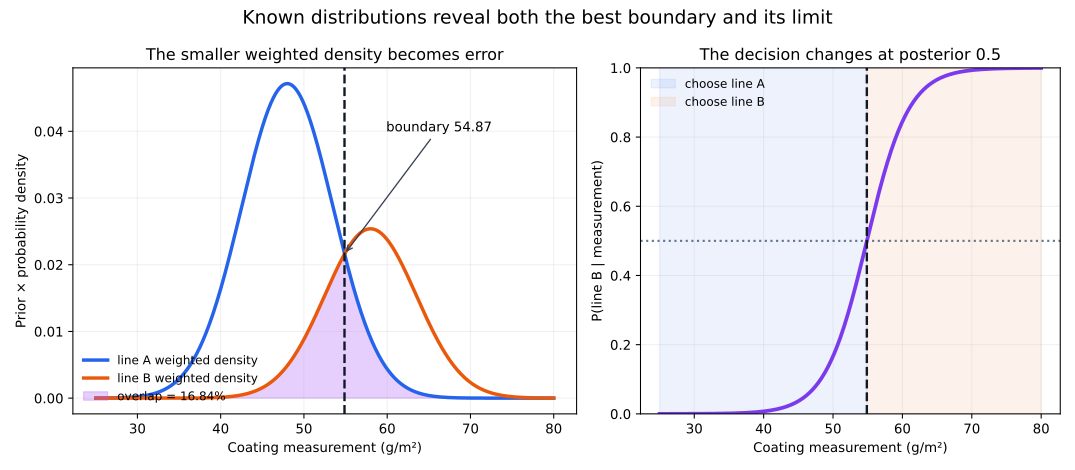
Read the left panel vertically at any measurement. The higher curve supplies the selected class, while the purple area under the lower curve supplies the unavoidable error. The right panel shows the same rule as a posterior probability: the choice changes when P(line B | measurement) crosses 0.5.

Compare the limit with a learned classifier

In a real task, the class means and standard deviations are usually unknown. A model estimates them from training data. scikit-learn’s GaussianNB documentation explains that the classifier assumes Gaussian feature likelihoods and estimates their means and variances from data.

Because this lesson has only one feature, the “naive” assumption that several features are conditionally independent does not affect the result. Fit the model on the 3,000 training rows and print what it learned:

from sklearn.naive_bayes import GaussianNB

train = measurements.query("split == 'train'").copy()
test = measurements.query("split == 'test'").copy()

learned_model = GaussianNB()
learned_model.fit(
    train[["coating_g_m2"]],
    train["production_line"],
)

model_parameters = pd.DataFrame({
    "class": learned_model.classes_,
    "prior": learned_model.class_prior_,
    "mean": learned_model.theta_[:, 0],
    "std": np.sqrt(learned_model.var_[:, 0]),
})
print(model_parameters.round(3).to_string(index=False))

 class  prior   mean   std
line_A   0.65 47.972 5.510
line_B   0.35 57.886 5.341

The learned values are close to the generator’s known values, but they are not identical. A finite random sample rarely reproduces every population parameter exactly.

Now compare the known Bayes rule with the learned model on the untouched test rows. The confusion matrix counts actual classes by row and predicted classes by column:

from sklearn.metrics import accuracy_score, confusion_matrix

known_predictions = bayes_predictions(
    test["coating_g_m2"].to_numpy()
)
learned_predictions = learned_model.predict(
    test[["coating_g_m2"]]
)

known_accuracy = accuracy_score(
    test["production_line"], known_predictions
)
learned_accuracy = accuracy_score(
    test["production_line"], learned_predictions
)
learned_matrix = confusion_matrix(
    test["production_line"],
    learned_predictions,
    labels=["line_A", "line_B"],
)

print(f"known Bayes rule test accuracy: {known_accuracy:.3f}")
print(f"learned GaussianNB test accuracy: {learned_accuracy:.3f}")
print(learned_matrix)

known Bayes rule test accuracy: 0.837
learned GaussianNB test accuracy: 0.839
[[588  62]
 [ 99 251]]

The first matrix row says that 588 actual line A sheets were classified as line A and 62 as line B. The second row says that 251 actual line B sheets were classified correctly and 99 were classified as line A. The model therefore made 161 mistakes among 1,000 test rows.

The learned model’s 83.9% test accuracy is slightly above the 83.16% expected Bayes accuracy. It did not defeat the Bayes rule. The Bayes value is a population expectation under the designed distributions; accuracy on one finite test set can fall above or below it by chance. The learned rule also scores 0.2 percentage points above the known rule on this particular test set, but the known rule remains optimal on average under the stated assumptions.

This distinction prevents a common reporting error. Bayes error is a population property under a specification. Test error is an estimate from one sample.

Common mistakes and troubleshooting

Integrating raw likelihoods without priors. The decision compares P(class) × density(x | class). Integrating the lower unweighted density silently assumes equal class priors and can move the boundary.

Treating a density height as a probability. A continuous variable has probability across an interval, represented by area. A density value can even exceed 1 when a distribution is very narrow, while its total area still equals 1.

Using a grid that misses the tails. The integration range must extend far enough beyond both means that the remaining density is negligible. Expand the range and increase the number of grid points; the reported error should stop changing at the precision you need.

Assuming every crossing pattern has one boundary. Equal standard deviations give one crossing here. Different standard deviations can produce two crossings, so keep all indices in changes and inspect the decision regions instead of always selecting changes[0].

Calling all model error irreducible. The 16.84% result is irreducible only when the classifier receives this one measurement and the assumptions are correct. A useful second feature could separate cases that overlap on coating alone. Poor preprocessing or a mismatched model can add avoidable error above the Bayes error.

Claiming that one test score changed the Bayes limit. A test set estimates performance with sampling noise. As the number of independent test cases grows, accuracy tends toward its expected value; a single test score can be higher or lower.

Using GaussianNB without checking the class shapes. Real measurements may be skewed, contain several peaks, or change over time. Inspect each class distribution and validate on representative later data. A theoretical answer from incorrect Gaussian assumptions is precise but not useful.

Adding dependent features without reconsidering the model. With several inputs, Gaussian Naive Bayes multiplies per-feature likelihoods under conditional independence. Strong dependence within a class can distort its probability estimates. Compare with another classifier and check probability calibration before using the probabilities in decisions. The probability calibration tutorial shows how to perform that check.

Forgetting the cost of each error. This lesson treats both mistakes equally. If confusing line B for line A matters more than the reverse, the best action minimizes expected cost rather than the raw count of errors. That requires cost-weighted decision regions.

Recap: separate model gaps from class overlap

Bayes error answers a narrow but valuable question: if the class distributions and priors were known, how often would the best rule still be wrong with the current information?

Keep this compact checklist:

• Calculate one likelihood curve per class.
• Multiply every likelihood by its class prior.
• Choose the largest weighted density at each input value.
• Integrate the smallest weighted density to measure expected error.
• Compare learned models with the limit across representative samples, not one lucky test result.
• Recalculate when features, priors, error costs, or distribution assumptions change.

For the fictional coating data, the weighted curves cross at 54.87 g/m². Their overlap produces 16.84% Bayes error and an expected accuracy limit of 83.16%. Gaussian Naive Bayes learned parameters close to the known values, while its 83.9% score on one test set illustrated normal sampling variation.

If priors, likelihoods, and posterior probabilities are still new, continue with calculating Bayes theorem from a frequency table in Python. The count-based view gives the same probability update without continuous densities.