Calibrate Gradient Boosting Probabilities in Python

A classifier can choose the correct label while giving an unreliable probability. Imagine that a device-monitoring model assigns a probability of 0.80 to an alert during the next seven days. If alerts occur for only half of the devices that receive probabilities near 0.80, the model is too confident. A maintenance team cannot treat that number as a reliable estimate of risk.

This tutorial shows how to diagnose and improve that problem. You will fit a gradient boosting classifier to fictional sensor readings, check its probabilities with a reliability diagram and two probability metrics, and apply sigmoid calibration with scikit-learn. The aim is not only to predict alert or no alert. It is to make a statement such as “about 30% risk” carry a useful numerical meaning.

This lesson assumes that you know the basic fit, predict, and train/test workflow. If those terms are new, start with your first machine learning model. You do not need previous knowledge of probability calibration.

Setup and reproducible data

You need Python 3.11 or later and a terminal, script editor, or notebook. Create a virtual environment, activate it, and install the four libraries used below:

python -m venv .venv
source .venv/bin/activate
python -m pip install numpy pandas scikit-learn matplotlib

On Windows PowerShell, use .venv\Scripts\Activate.ps1 for the activation step. The published results were executed with Python 3.13.2, NumPy 2.5.1, pandas 3.0.3, scikit-learn 1.9.0, and Matplotlib 3.11.0.

The lesson uses device_alerts.csv, an original synthetic dataset released as CC0-1.0. Its 3,000 device records are fictional. A fixed NumPy seed generates the sensor values and outcomes, so the complete build is reproducible. Synthetic data is useful here because it avoids publishing real maintenance or customer information, but its results should not be treated as evidence about real equipment.

Load the file and inspect a small selection of columns first:

import pandas as pd

devices = pd.read_csv(
    "https://datatweets.com/datasets/blog/calibrate-gradient-boosting-probabilities-python/device_alerts.csv"
)

devices[[
    "device_id", "temperature_c", "vibration_mm_s",
    "errors_24h", "alert_next_7_days",
]].head()

  device_id  temperature_c  vibration_mm_s  errors_24h  alert_next_7_days
0    DV-0001           40.2            2.20           1                    0
1    DV-0002           52.3            9.01           1                    1
2    DV-0003           34.9            3.66           1                    0
3    DV-0004           42.9            6.03           1                    1
4    DV-0005           46.7            0.80           0                    0

Each row represents one device at one observation time. The features are measurements available to the model: device age, temperature, vibration, recent errors, and days since service. The target is alert_next_7_days: 1 means an alert occurred during the following seven days, and 0 means it did not.

Check the target balance before modeling:

print(devices.shape)
print(devices["alert_next_7_days"].value_counts())
print(f"alert rate: {devices['alert_next_7_days'].mean():.3f}")

(3000, 7)
alert_next_7_days
0    2224
1     776
Name: count, dtype: int64
alert rate: 0.259

About 25.9% of the observations are followed by an alert. This base rate, or overall event frequency, matters: a probability of 0.40 is above the average risk in this dataset even though it is below the common 0.50 classification threshold.

The mental model: confidence should match frequency

A model is calibrated when predicted probabilities agree with observed frequencies. Among many cases assigned a probability near 0.20, an alert should occur about 20% of the time. Among cases near 0.70, the observed rate should be about 70%.

Calibration is different from classification accuracy. Accuracy checks whether a final class label is correct. It does not ask whether 0.51 and 0.99 describe different levels of confidence honestly. Two models can make the same labels at a 0.50 threshold while reporting very different probabilities.

A reliability diagram, also called a calibration curve, checks the connection between confidence and frequency:

1. Sort test predictions into probability groups, or bins.
2. Find the mean predicted probability in each bin.
3. Find the fraction of real alerts in the same bin.
4. Plot predicted probability against observed alert rate.

Perfect agreement follows the diagonal line observed rate = predicted probability. A point below that line means the mean predicted risk in that bin is higher than the observed event rate. A point above it means the mean predicted risk is lower than the observed rate.

Calibration cannot make an uninformative model useful. A classifier must first separate higher-risk cases from lower-risk cases. Calibration then adjusts how its scores map to probabilities.

Fit a gradient boosting baseline

Reserve 25% of the rows for one final test set. stratify keeps almost the same alert rate in both parts, and random_state makes the split repeatable:

from sklearn.model_selection import train_test_split

features = [
    "device_age_days",
    "temperature_c",
    "vibration_mm_s",
    "errors_24h",
    "days_since_service",
]

train, test = train_test_split(
    devices,
    test_size=0.25,
    random_state=63,
    stratify=devices["alert_next_7_days"],
)

X_train = train[features]
y_train = train["alert_next_7_days"]
X_test = test[features]
y_test = test["alert_next_7_days"]

print(len(train), len(test))

2250 750

The next step fits a histogram-based gradient boosting classifier. Gradient boosting builds a sequence of small decision trees, with later trees correcting errors left by earlier trees. The histogram version groups continuous feature values into bins to train efficiently.

from sklearn.ensemble import HistGradientBoostingClassifier

base_model = HistGradientBoostingClassifier(
    learning_rate=0.09,
    max_iter=180,
    max_leaf_nodes=15,
    min_samples_leaf=18,
    l2_regularization=0.2,
    random_state=63,
)
base_model.fit(X_train, y_train)

raw_probability = base_model.predict_proba(X_test)[:, 1]
print(raw_probability[:5].round(3))

[0.041 0.352 0.177 0.629 0.174]

predict_proba returns one column per class. [:, 1] selects the estimated probability of class 1, which is an alert. These numbers are model estimates, not guaranteed event frequencies. We must test them.

Measure probability quality

Use metrics that evaluate probabilities rather than only class labels. Brier loss is the mean squared difference between each predicted probability and its zero-or-one outcome. Log loss gives a larger penalty to confident predictions that are wrong. Lower is better for both metrics.

The following helper also reports accuracy after turning probabilities at or above 0.50 into alert labels:

import pandas as pd
from sklearn.metrics import accuracy_score, brier_score_loss, log_loss

def probability_metrics(name, actual, probability):
    predicted = (probability >= 0.5).astype(int)
    return {
        "model": name,
        "brier": brier_score_loss(actual, probability),
        "log_loss": log_loss(actual, probability),
        "accuracy": accuracy_score(actual, predicted),
    }

baseline_metrics = probability_metrics(
    "uncalibrated", y_test, raw_probability
)
pd.DataFrame([baseline_metrics]).round(4)

          model   brier  log_loss  accuracy
0  uncalibrated  0.1685    0.5199     0.752

These numbers establish a comparison point. Brier loss combines calibration and the model’s ability to separate cases, so it should not be read as a pure calibration measure by itself. We will compare the same underlying model before and after calibration and also inspect the reliability diagram.

Calibrate without leaking test answers

A calibrator is a small model that learns how to transform a classifier’s scores into better probability estimates. It must learn from predictions for rows that the base classifier did not train on. If it sees predictions for the same rows used to fit the classifier, those scores can look unrealistically good and produce a biased mapping.

CalibratedClassifierCV creates the required separation with cross-validation. With five folds and ensemble=False, scikit-learn performs this process:

1. Divide the 2,250 training rows into five folds.
2. Repeatedly fit the base estimator on four folds and predict the held-out fold.
3. Join those out-of-fold predictions and fit the calibrator to them.
4. Fit one final base estimator on all 2,250 training rows for later predictions.

The untouched test set is not used in any of these steps. The official scikit-learn probability calibration guide explains why calibration data should be independent of the data used to fit the classifier.

Use sigmoid calibration, which applies a two-parameter sigmoid function to the classifier’s scores. It is a practical starting choice and is less flexible than isotonic calibration:

from sklearn.calibration import CalibratedClassifierCV

calibrated_model = CalibratedClassifierCV(
    estimator=HistGradientBoostingClassifier(
        learning_rate=0.09,
        max_iter=180,
        max_leaf_nodes=15,
        min_samples_leaf=18,
        l2_regularization=0.2,
        random_state=63,
    ),
    method="sigmoid",
    cv=5,
    ensemble=False,
)
calibrated_model.fit(X_train, y_train)

calibrated_probability = calibrated_model.predict_proba(X_test)[:, 1]

Now compare both sets of probabilities on exactly the same 750 test rows:

comparison = pd.DataFrame([
    probability_metrics("uncalibrated", y_test, raw_probability),
    probability_metrics(
        "sigmoid calibrated", y_test, calibrated_probability
    ),
])
print(comparison.round(4).to_string(index=False))

             model  brier  log_loss  accuracy
      uncalibrated 0.1685    0.5199    0.7520
sigmoid calibrated 0.1605    0.4897    0.7707

The calibrated model has lower Brier loss and lower log loss on this test set. Its accuracy also rises because the mapping moves some probabilities across 0.50, but accuracy improvement is not calibration’s main purpose. A different dataset could improve probability quality without changing any labels.

Inspect a few rows to make that distinction concrete:

preview = pd.DataFrame({
    "device_id": test["device_id"].iloc[:5].to_numpy(),
    "actual": y_test.iloc[:5].to_numpy(),
    "raw_probability": raw_probability[:5].round(3),
    "calibrated_probability": calibrated_probability[:5].round(3),
})
print(preview.to_string(index=False))

device_id  actual  raw_probability  calibrated_probability
  DV-1278       0            0.041                   0.110
  DV-1708       1            0.352                   0.342
  DV-2777       0            0.177                   0.235
  DV-2158       1            0.629                   0.497
  DV-0464       1            0.174                   0.233

Calibration does not simply increase every probability. In this fitted mapping, it raises some low estimates and lowers some high estimates. For DV-2158, the value moves from 0.629 to 0.497, which also changes the label at a 0.50 threshold. One row cannot show that either estimate is better; calibration is evaluated across many cases.

Draw and read a reliability diagram

The next code groups each probability set into eight bins with similar numbers of rows. With 750 test devices, each bin contains about 93 or 94 devices. strategy="quantile" avoids creating a few nearly empty groups when predictions are unevenly distributed.

from sklearn.calibration import calibration_curve

raw_observed, raw_mean = calibration_curve(
    y_test, raw_probability, n_bins=8, strategy="quantile"
)
cal_observed, cal_mean = calibration_curve(
    y_test, calibrated_probability, n_bins=8, strategy="quantile"
)

print("raw:       ", raw_mean.round(3))
print("observed:  ", raw_observed.round(3))
print("calibrated:", cal_mean.round(3))

raw:        [0.011 0.037 0.076 0.123 0.195 0.319 0.497 0.781]
observed:   [0.053 0.096 0.161 0.149 0.255 0.387 0.383 0.585]
calibrated: [0.052 0.103 0.151 0.194 0.247 0.323 0.422 0.619]

The last raw bin has a mean predicted probability of 0.781, but its observed alert rate is 0.585. That is overconfidence. After calibration, the bin’s mean prediction is 0.619, much closer to the same observed rate. At the low end, a raw mean of 0.011 understates an observed rate of 0.053; calibration moves the mean prediction to 0.052.

The observed rates are the same for the raw and calibrated curves in each quantile bin here. This fitted sigmoid mapping preserves the order of the predictions, so the same devices remain together while their probability values change.

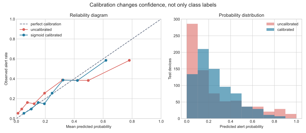
Read the left panel by comparing each colored point with the dashed diagonal. The calibrated blue curve is generally closer, especially at the lowest and highest probabilities. The right panel shows how the estimates changed: sigmoid calibration pulls many extreme estimates toward the middle. It changes reported confidence and can also change final labels.

Do not expect a perfectly straight empirical curve. Each point is estimated from a limited number of test rows, and another sample would produce slightly different observed rates. For a production system, evaluate calibration on recent data and add uncertainty estimates when decisions are sensitive.

Common mistakes and troubleshooting

Calibrating and evaluating on the same held-out rows. If you fit a calibrator on the test set and then report its test metrics, the evaluation is no longer independent. Use cross-validation inside the training set, as this tutorial does, or maintain separate training, calibration, and test sets.

Using accuracy to judge probability quality. Accuracy discards how confident the predictions were. Report a probability metric such as Brier loss or log loss and inspect a reliability diagram. Also remember that Brier loss reflects more than calibration alone.

Choosing too many bins for a small test set. More bins give each point fewer rows, so the observed rate becomes noisy. The current calibration_curve documentation notes that empty bins are omitted. Start with 5 to 10 bins and check how many observations support each one.

Assuming sigmoid is always best. Sigmoid calibration makes a specific S-shaped adjustment. Isotonic calibration is more flexible, but scikit-learn warns that it tends to overfit when there are far fewer than 1,000 calibration samples. Compare methods with validation data rather than choosing one after inspecting the final test result.

Treating a calibrated score as a decision rule. A probability and an action threshold solve different problems. A maintenance team may inspect devices above 0.30 if missing an alert is costly, or use a higher threshold if inspections are limited. Choose that threshold from costs and validation data, not because 0.50 is the default.

Ignoring change over time. Calibration can drift when device types, sensors, service policies, or alert definitions change. Monitor the observed event rate and reliability curve on new labeled data. Refit only through a documented process that preserves a final evaluation set.

If results differ, confirm the package versions, use the published CSV, keep random_state=63, and copy the same model settings. Small numerical differences can still occur across platforms. A missing predict_proba method also means the chosen base estimator cannot supply the probabilities expected by this workflow.

Recap

Probability calibration asks a precise question: when a classifier says p, does the event occur about p of the time for similar predictions? A reliability diagram compares mean predicted probabilities with observed rates, while Brier loss and log loss summarize probability errors in complementary ways.

In this synthetic device-alert example, the raw gradient boosting model was too extreme in several probability ranges. Five-fold sigmoid calibration learned from out-of-fold training predictions, leaving all 750 test rows untouched. On that test set, Brier loss fell from 0.1685 to 0.1605 and log loss fell from 0.5199 to 0.4897.

The durable workflow is: split first, fit the classifier, learn calibration only from independent predictions, and evaluate probabilities once on untouched data. Calibration makes confidence easier to use, but it does not replace good features, representative data, threshold design, or monitoring after deployment.