How to Check ARIMA Residuals with Ljung-Box Tests in Python

A fitted ARIMA model can produce a smooth forecast and a reasonable error score while still missing a repeatable pattern. The missed pattern appears in its residuals: the differences between observed and fitted values.

To check ARIMA residuals in Python, remove any state-initialization residuals, inspect a residual autocorrelation (ACF) plot, and run acorr_ljungbox() at relevant lags with model_df=p+q. Large ACF spikes or a small Ljung-Box p-value show that the model left time dependence unexplained; a large p-value means the test did not find such evidence, not that the model is certainly correct.

We will make that distinction visible by fitting two models to fictional daily energy-meter readings. One model intentionally ignores the relationship between recent days. The other represents two earlier daily changes and should leave less structure behind.

Prerequisites and Setup

You need Python 3 and a way to run a Python file or notebook cell. You do not need previous experience with statistical tests. Basic pandas knowledge is helpful, but each important term is defined when it first appears.

Create a virtual environment, activate it, and install the packages used by the published environment:

python -m venv .venv
source .venv/bin/activate
python -m pip install numpy pandas statsmodels matplotlib

On Windows PowerShell, activate the environment with .venv\Scripts\Activate.ps1. The published run used Python 3.13.2, NumPy 2.5.1, pandas 3.0.3, statsmodels 0.14.6, and Matplotlib 3.11.0.

Download building_energy_meter.csv and save it beside your Python file. It contains 240 complete daily readings from a fictional building’s cumulative energy meter. The data was generated with a fixed random seed for this lesson and is released under CC0-1.0. It does not measure a real building.

The chart will be saved to a file, so select Matplotlib’s headless Agg backend before importing pyplot:

import matplotlib

matplotlib.use("Agg")

import matplotlib.pyplot as plt
import pandas as pd
from statsmodels.graphics.tsaplots import plot_acf
from statsmodels.stats.diagnostic import acorr_ljungbox
from statsmodels.tsa.arima.model import ARIMA

This import order works on a server or automated job without a desktop display.

Understanding What Residual Checks Measure

A residual is what remains after subtracting a fitted value from the observed value:

residual at time t = observed value at time t - fitted value at time t

If a model has captured the useful time pattern, its residuals should behave approximately like white noise. In this context, that means the residuals are not correlated with their earlier values. Their mean should also be near zero, and their spread should be reasonably stable over time.

An autocorrelation measures how strongly a series is related to an earlier copy of itself. Lag 1 compares neighboring days. Lag 7 compares values one week apart. A residual ACF plot shows these correlations across several lags.

The Ljung-Box test checks several residual correlations together. Its null hypothesis, the starting claim tested by the calculation, is that every residual autocorrelation from lag 1 through the requested lag is zero. We will use a 5% decision threshold:

• p < 0.05: reject the no-autocorrelation claim; the residuals contain evidence of time structure.
• p >= 0.05: do not reject the claim; this test did not find enough evidence of autocorrelation through that lag.

The second statement is deliberately cautious. A test can miss weak structure, and a model can fail for reasons that autocorrelation does not measure. The test does not check changing variance, unusual outliers, data leakage, or future forecast accuracy.

We will request lags 5, 10, and 20. These give short, medium, and longer views of this daily process. Choose lags from the process and forecast horizon before reading the results. If a real operation has a weekly pattern, include lag 7 or a multiple of 7 rather than copying this list without thought.

Load the Meter Readings and Reveal Daily Change

First, parse the dates, sort them, and check for duplicate dates. Then use asfreq("D") to give the series an explicit daily frequency. Any missing calendar dates will appear as missing values.

meter = pd.read_csv(
    "building_energy_meter.csv",
    parse_dates=["date"],
)
meter = meter.sort_values("date").set_index("date")
series = meter["cumulative_energy_kwh"].asfreq("D")

print(series.head(8).to_string())
print("\nrows:", len(series))
print("frequency:", pd.infer_freq(series.index))
print("duplicate dates:", meter.index.duplicated().sum())
print("missing readings:", series.isna().sum())

The executed output is:

date
2025-01-01    12546.73
2025-01-02    12597.93
2025-01-03    12652.01
2025-01-04    12706.77
2025-01-05    12762.44
2025-01-06    12813.34
2025-01-07    12865.10
2025-01-08    12914.40
Freq: D

rows: 240
frequency: D
duplicate dates: 0
missing readings: 0

The index is complete, unique, and daily. Those checks matter because “lag 10” represents ten days only when the rows are correctly spaced.

The meter is cumulative, so its level always rises. An ARIMA model with d=1 works with one difference, calculated as the current reading minus the previous reading. Here, that difference is one day’s energy use.

Inspect a few differences before fitting the model:

daily_change = series.diff().dropna()

print(daily_change.head(6).round(2).to_string())
print("\nmean daily change:", round(daily_change.mean(), 2), "kWh")

date
2025-01-02    51.20
2025-01-03    54.08
2025-01-04    54.76
2025-01-05    55.67
2025-01-06    50.90
2025-01-07    51.76
Freq: D

mean daily change: 51.57 kWh

The differences move around a stable positive level. They are not independent, however: nearby days were generated with a short memory. Our residual checks should reveal whether a fitted model captures it.

Fit an Underfit Model and a Two-Lag Model

ARIMA uses the order (p, d, q). p is the number of autoregressive terms, d is the number of differences, and q is the number of moving-average error terms. A moving-average error term is not a rolling average of the meter readings.

The first candidate, ARIMA(0,1,0), models a constant average daily change but no dependence between changes. The second, ARIMA(2,1,0), lets the current change depend on the previous two changes.

Fit both with a time trend. In an integrated model with d=1, trend="t" supplies drift to the differenced process. The current statsmodels ARIMA reference documents the (p,d,q) order and notes that an integrated model has no trend by default.

model_specs = {
    "Drift only ARIMA(0,1,0)": (0, 1, 0),
    "ARIMA(2,1,0)": (2, 1, 0),
}

fitted_models = {
    label: ARIMA(series, order=order, trend="t").fit()
    for label, order in model_specs.items()
}

for label, fitted in fitted_models.items():
    print(f"{label}: AIC={fitted.aic:.2f}")

Drift only ARIMA(0,1,0): AIC=1284.76
ARIMA(2,1,0): AIC=1214.23

Akaike information criterion (AIC) balances in-sample fit against model complexity; a lower value is preferred when models use the same observations and target. The two-lag model has the lower AIC, but AIC alone does not tell us whether its residual correlations are acceptably small. That is the next question.

Remove Initialization Effects Before Testing

Statsmodels fits ARIMA through a state-space calculation. The first residual can be affected by the model’s initial estimate of its internal state. Testing that value as if it were an ordinary fitted error can distort a diagnostic.

The model result records how many early values to exclude. Use the larger of loglikelihood_burn and nobs_diffuse, then keep the remaining residuals:

residual_sets = {}

for label, fitted in fitted_models.items():
    burn = max(fitted.loglikelihood_burn, fitted.nobs_diffuse)
    residual_sets[label] = fitted.resid.iloc[burn:]
    print(f"{label}: removed {burn}, kept {len(residual_sets[label])}")

Drift only ARIMA(0,1,0): removed 1, kept 239
ARIMA(2,1,0): removed 1, kept 239

Statsmodels’ official test_serial_correlation() documentation uses the same principle: it ignores the initial residuals controlled by the state-space burn and diffuse periods.

Now summarize each residual series. The lag-1 value is the correlation between each residual and the preceding day’s residual.

for label, residuals in residual_sets.items():
    print(
        f"{label}: mean={residuals.mean():.3f}, "
        f"sd={residuals.std():.3f}, "
        f"lag-1 ACF={residuals.autocorr(1):.3f}"
    )

Drift only ARIMA(0,1,0): mean=0.000, sd=3.534, lag-1 ACF=0.470
ARIMA(2,1,0): mean=0.003, sd=3.022, lag-1 ACF=-0.029

Both means are close to zero. The important contrast is lag 1: 0.470 is substantial remaining correlation, while -0.029 is close to zero. The two-lag model also has a smaller residual standard deviation, but we still need a joint check across more than one lag.

Run Ljung-Box Tests with Correct Degrees of Freedom

The Ljung-Box calculation must account for parameters already estimated by the model. The statsmodels acorr_ljungbox() reference recommends model_df=p+q for an ARMA error process. It subtracts this value from each requested lag’s test degrees of freedom.

Build one result table for both models. The differencing order d is not included in model_df here.

test_rows = []

for label, order in model_specs.items():
    model_df = order[0] + order[2]
    result = acorr_ljungbox(
        residual_sets[label],
        lags=[5, 10, 20],
        model_df=model_df,
        return_df=True,
    )

    for lag, row in result.iterrows():
        test_rows.append({
            "model": label,
            "lag": lag,
            "model_df": model_df,
            "lb_stat": row["lb_stat"],
            "lb_pvalue": row["lb_pvalue"],
        })

ljung_box = pd.DataFrame(test_rows)
print(
    ljung_box.to_string(
        index=False,
        formatters={
            "lb_stat": "{:.2f}".format,
            "lb_pvalue": "{:.3g}".format,
        },
    )
)

The executed table is:

                    model  lag  model_df lb_stat lb_pvalue
Drift only ARIMA(0,1,0)     5         0   65.49  8.88e-13
Drift only ARIMA(0,1,0)    10         0   76.01  3.03e-12
Drift only ARIMA(0,1,0)    20         0  101.99  5.53e-13
             ARIMA(2,1,0)     5         2    7.01    0.0714
             ARIMA(2,1,0)    10         2   13.95    0.0832
             ARIMA(2,1,0)    20         2   24.31     0.145

At every requested lag, the drift-only p-value is far below 0.05. We reject the no-autocorrelation claim: that model has missed time structure.

The ARIMA(2,1,0) p-values are 0.0714, 0.0832, and 0.145. None falls below the chosen threshold, so these tests do not find enough evidence of residual autocorrelation. The lag-5 result is only slightly above 0.05, so it should not be described as a perfect pass. More data or a different preselected horizon could change the conclusion.

Also ensure that every requested lag is greater than model_df. If lag - model_df is zero or negative, statsmodels returns a missing p-value because the adjusted test has no positive degrees of freedom.

See What the Test Compresses into One Number

A p-value is a compact decision aid, not a picture of the remaining pattern. Plot the residual ACF as well. Set bartlett_confint=False so plot_acf() uses confidence limits based on a white-noise residual assumption, as described in the official plot_acf() documentation.

The core plotting calls below create the two lower panels of the published diagnostic figure:

fig, axes = plt.subplots(1, 2, figsize=(10, 4))

for axis, (label, residuals) in zip(axes, residual_sets.items()):
    plot_acf(
        residuals,
        lags=20,
        alpha=0.05,
        zero=False,
        bartlett_confint=False,
        title="",
        ax=axis,
    )
    axis.set_title(label)
    axis.set_xlabel("Lag (days)")
    axis.set_ylabel("Residual autocorrelation")

fig.tight_layout()
fig.savefig("arima_residual_acf.svg", format="svg")
plt.close(fig)

The published chart adds the original meter series and its first differences above those residual ACF panels. It is the real SVG generated by the executed lesson build:

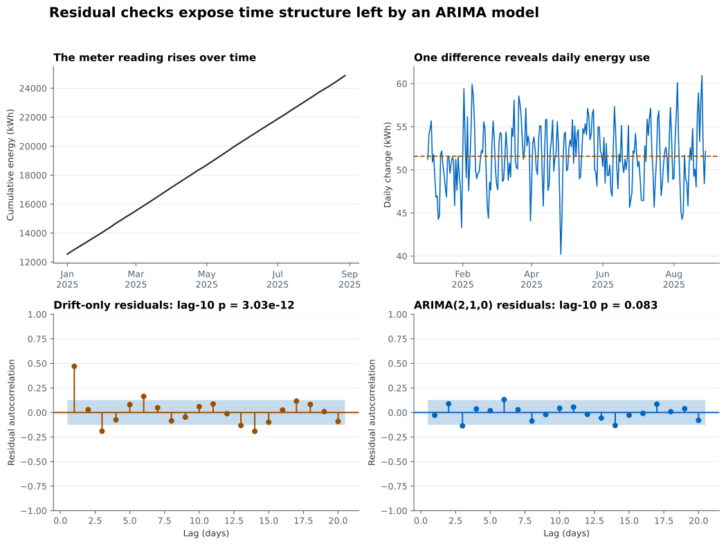
Read the lower-left panel first. Its lag-1 bar is well outside the shaded approximate 95% confidence band, and later bars show a decaying pattern. The drift-only model repeatedly makes errors in the same direction because it has not represented the two-day memory.

The lower-right bars are shorter and move around zero without the same clear shape. This visual agrees with the larger Ljung-Box p-values. Agreement between a plot and a formal test is more informative than either output viewed alone.

Common Mistakes and Troubleshooting

Testing the observations instead of the residuals. acorr_ljungbox(series) asks whether the original meter readings are autocorrelated. That is not the diagnostic question. Pass the fitted model’s cleaned residuals.

Keeping state-initialization errors. A very large first residual can dominate the scale and affect tests. Remove the number reported by the fitted state-space result, or use ARIMAResults.test_serial_correlation(), which handles its initial burn internally.

Leaving model_df=0 for every model. When an ARIMA model includes AR or MA terms, it estimates those parameters from the same data. Use p+q for the standard adjustment, and do not request lags that are too small after that subtraction.

Treating p >= 0.05 as proof of white noise. The correct statement is that the test did not reject its null hypothesis at the chosen threshold. Check the residual plot, ACF, variance over time, outliers, and results on later data.

Trying orders until one p-value passes. Repeatedly changing a model after reading the same diagnostic makes the final p-value harder to interpret. Use diagnostics to identify a plausible problem, change the specification for a reason, and then evaluate forecasts on untouched later observations.

Ignoring seasonal lags. A clean ACF through lag 10 says little about a monthly pattern in daily data. Select lags that can expose known operating cycles and leave enough observations for a useful test.

Using irregular dates as regular lags. Ten rows are not ten days when dates are missing or duplicated. Sort the index, check duplicates, set the expected frequency, and decide how unknown readings should be handled before fitting.

Replacing forecast evaluation with residual checks. Clean in-sample residuals do not guarantee accurate future predictions. Compare candidate orders on later timestamps, as shown in this leakage-safe autoregressive forecasting workflow, and keep a simple baseline on the same dates.

Expecting Ljung-Box to detect every problem. It targets linear autocorrelation. A residual series can pass while its variance changes over time or while rare events create unsafe errors. Add diagnostics that match the risks of your application.

Recap: Pass Diagnostics, Then Test Forecasts

Residual checking asks a precise question: after fitting the model, is any repeatable time relationship still visible in its errors?

The reliable workflow is to remove initialization effects, look at residuals over time, inspect their ACF, and run Ljung-Box tests at preselected lags. Adjust the test with model_df=p+q, and interpret the p-value as evidence rather than a certificate.

In this synthetic example, ARIMA(0,1,0) left lag-1 residual autocorrelation of 0.470 and failed the lag-10 test with p = 3.03e-12. ARIMA(2,1,0) reduced lag-1 residual autocorrelation to -0.029; its lag-10 test returned p = 0.083, so the chosen check did not reject no autocorrelation.

That is enough to rule out the drift-only specification as an adequate model and keep the two-lag model as a candidate. It is not enough to deploy it. The next step is to compare both models with a simple baseline on later, untouched dates. If the data has a regular weekly cycle, first establish the reference point with a seasonal naive forecast in Python and require the ARIMA model to improve on it under the same forecast horizon.