How to Compare Data Scalers with Cross-Validation in Python

Should you use StandardScaler, RobustScaler, or no scaler at all? A chart of the raw columns can suggest reasonable choices, but it cannot tell you which one will help your model predict new rows more accurately.

To choose a data scaler in scikit-learn, put the scaler and model in one Pipeline, list the scaler candidates in a GridSearchCV parameter grid, and fit the search only on the training data. Compare the mean cross-validation error, keep a separate test set untouched during selection, and use that test set once to check the selected pipeline.

This tutorial applies that method to a distance-based regression model. You will see all nine measured candidates, not only the winner, and learn what the results do and do not show about outliers.

Setup and the fictional service visits

You need Python 3.11 or newer and a basic understanding of rows and columns. A pandas DataFrame is a table stored in memory. You do not need previous experience with feature scaling, K-nearest neighbors, or cross-validation; each term is introduced before it is used.

Create a virtual environment, activate it, and install the four packages used in the lesson:

python -m venv .venv
source .venv/bin/activate
python -m pip install numpy pandas scikit-learn matplotlib

On Windows PowerShell, activate the environment with .venv\Scripts\Activate.ps1. The published build ran with Python 3.13.2, NumPy 2.5.1, pandas 3.0.3, scikit-learn 1.9.0, and Matplotlib 3.11.0.

Download service_visits.csv and save it beside your Python file or notebook. This is an original synthetic dataset created for this lesson and released under CC0-1.0. All 1,200 visit IDs, measurements, extreme observations, and durations are fictional.

Each row describes a technician’s completed service visit. The five input features are travel distance, equipment count, site area, access waiting time, and years since the previous service. The value to predict, called the target, is the visit duration in minutes.

Load the file and display a small sample before making any modeling decision:

import pandas as pd

visits = pd.read_csv("service_visits.csv")
print(visits.head().to_string(index=False))
print("shape:", visits.shape)

The first five rows and the table size are:

visit_id  travel_km  equipment_count  site_area_m2  access_wait_min  years_since_service  visit_duration_min
 SV-0001       8.74                6         842.0             4.70                 7.12               145.7
 SV-0002       8.48                9        3420.1             1.26                 6.50               214.2
 SV-0003       8.38                4         592.8             2.76                 6.99                98.4
 SV-0004       7.56                5         313.2            13.58                 2.10               123.2
 SV-0005       9.03                4         192.5             6.77                 5.01                92.6
shape: (1200, 7)

The target appears in the seventh column. visit_id identifies a row for people reading the file; it is not a measured property of a visit, so it will not become a model feature.

How feature scaling works in a neighbor search

A feature scaler changes the center and spread of each numeric column. It does not create new information. For example, it can express square metres and years on comparable numeric scales while preserving the order of the values within each feature.

This matters for K-nearest neighbors, or KNN. To predict one row, a KNN regressor finds the k training rows with the smallest numerical distance from it and averages their target values. If site area differs by 400 and equipment count differs by 1, the raw distance is driven mainly by 400—even if one extra piece of equipment is important to visit duration.

The three routes in this lesson make different choices:

• No scaling passes every raw number directly to KNN.
• StandardScaler subtracts each training column’s mean and divides by its standard deviation.
• RobustScaler subtracts each training column’s median and divides by its interquartile range, or IQR. The IQR is the distance between the 25th and 75th percentiles.

The current scikit-learn StandardScaler documentation notes that its mean and standard deviation are sensitive to outliers. The RobustScaler documentation explains that medians and IQRs are less influenced by extreme values. That difference makes both scalers reasonable candidates here, but it does not tell us which one will predict better.

Reserve the final check before comparing anything

First select the five model features and the target. Then hold out 20% of the rows with a fixed random seed:

from sklearn.model_selection import train_test_split

features = [
    "travel_km",
    "equipment_count",
    "site_area_m2",
    "access_wait_min",
    "years_since_service",
]
X = visits[features]
y = visits["visit_duration_min"]

X_train, X_test, y_train, y_test = train_test_split(
    X,
    y,
    test_size=0.2,
    random_state=20260719,
)
print(X_train.shape, X_test.shape)

The split leaves 960 rows for selection and 240 for the final check:

(960, 5) (240, 5)

Do not inspect test errors while choosing a scaler. Repeatedly choosing whatever performs best on the test set would turn that set into another validation set. Its score would no longer be a clean final check.

Now inspect the ranges in X_train only. The median provides a typical central value without being pulled as strongly by extreme rows:

feature_ranges = X_train.agg(["min", "median", "max"]).T
feature_ranges.columns = ["minimum", "median", "maximum"]
print(feature_ranges.round(2).to_string())

The training ranges show why distances calculated from the raw values need attention:

                     minimum  median  maximum
travel_km               0.50   11.35    48.00
equipment_count         1.00    5.00    15.00
site_area_m2           45.00  410.25  6461.50
access_wait_min         0.00    3.47   108.84
years_since_service     0.11    3.96     7.99

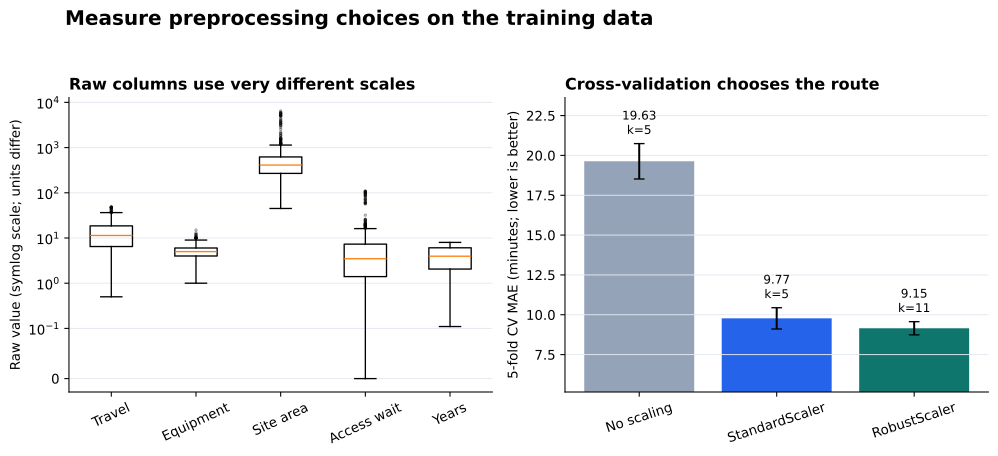
Site area reaches 6,461.5, while years since service never reaches 8. Access waits also have a long upper tail: the median is 3.47 minutes, but the maximum is 108.84. These are legitimate fictional observations in this dataset, not missing-value codes.

Make preprocessing part of the candidate

Cross-validation estimates performance by repeatedly fitting on part of the training data and validating on another part. Five-fold cross-validation divides the 960 training rows into five parts. Each run fits on four parts and validates on the fifth, so every row is used for validation once.

The scaler must be fit separately inside each fold. If you scale all 960 rows first and then cross-validate, every validation fold influences the mean, standard deviation, median, or IQR used to transform the corresponding training folds. That is data leakage: information crosses a boundary that the evaluation is meant to protect.

A scikit-learn Pipeline keeps the scaler and model together. Start with a named placeholder for the scaler, followed by KNN:

from sklearn.neighbors import KNeighborsRegressor
from sklearn.pipeline import Pipeline

pipeline = Pipeline([
    ("scale", "passthrough"),
    ("model", KNeighborsRegressor()),
])

"passthrough" means “leave this step inactive.” The Pipeline API allows a full step to be replaced with another transformer or with "passthrough". That lets one parameter grid compare preprocessing choices as complete workflows.

Next, create a shuffled KFold object with a fixed seed. These fictional visits are independent and have no time order or repeated customer groups, so shuffled folds match the scenario. Search three scaler choices and three values of n_neighbors:

from sklearn.model_selection import GridSearchCV, KFold
from sklearn.preprocessing import RobustScaler, StandardScaler

folds = KFold(
    n_splits=5,
    shuffle=True,
    random_state=20260719,
)

search = GridSearchCV(
    estimator=pipeline,
    param_grid={
        "scale": [
            "passthrough",
            StandardScaler(),
            RobustScaler(),
        ],
        "model__n_neighbors": [5, 11, 21],
    },
    scoring="neg_mean_absolute_error",
    cv=folds,
    n_jobs=1,
    refit=True,
)
search.fit(X_train, y_train)

model__n_neighbors uses two underscores because the n_neighbors setting belongs to the pipeline step named model. Testing the neighbor count together with the scaler is fairer than fixing a value that may suit only one scaling method.

Mean absolute error (MAE) is the average absolute distance between each predicted duration and its true duration. It stays in minutes, and lower is better. scikit-learn uses a negative MAE scorer because its search tools consistently treat larger scores as better; we will reverse the sign when displaying the result.

Read the comparison, not only the winning row

GridSearchCV stores one row per candidate in cv_results_. The next code gives the scaler objects readable names, converts the scores back to positive MAE, and sorts all nine candidates from lowest error to highest:

def scaler_name(value):
    if value == "passthrough":
        return "No scaling"
    return type(value).__name__


candidates = pd.DataFrame(search.cv_results_)
candidates["scaler"] = candidates["param_scale"].map(scaler_name)
candidates["neighbors"] = candidates[
    "param_model__n_neighbors"
].astype(int)
candidates["cv_mae_min"] = -candidates["mean_test_score"]
candidates["cv_mae_std_min"] = candidates["std_test_score"]

shown = candidates.sort_values("cv_mae_min")[[
    "scaler",
    "neighbors",
    "cv_mae_min",
    "cv_mae_std_min",
]]
print(shown.round(3).to_string(index=False))

The executed five-fold results are:

        scaler  neighbors  cv_mae_min  cv_mae_std_min
  RobustScaler         11       9.152           0.414
  RobustScaler          5       9.542           0.312
  RobustScaler         21       9.613           0.343
StandardScaler          5       9.774           0.668
StandardScaler         11       9.905           0.330
StandardScaler         21      10.411           0.547
    No scaling          5      19.630           1.110
    No scaling         11      20.647           1.083
    No scaling         21      21.512           1.227

Read one row at a time. RobustScaler with 11 neighbors has the lowest mean validation MAE: 9.152 minutes. The 0.414 value is the standard deviation of the five fold-level MAE values, so the errors were not identical across folds.

The comparison also shows a broader pattern. Every scaled candidate performs much better than every unscaled candidate. That result is consistent with how KNN handles columns whose raw ranges differ by thousands, but the measured size of the difference belongs to this dataset and model.

Within the scaled candidates, the gap is smaller. The best robust-scaled route is 0.622 minutes lower than the best standard-scaled route in mean cross-validation MAE. This result supports selecting the robust route, but it is not a universal statement that RobustScaler always wins when a dataset has outliers.

The generated chart connects the raw ranges to the measured comparison. The error bars show variation across folds, not uncertainty for every future service visit.

Use the held-out rows once

With refit=True, GridSearchCV fits the winning pipeline again on all 960 training rows. Confirm its two selected settings before using the test set:

print("scaler:", type(search.best_params_["scale"]).__name__)
print("neighbors:", search.best_params_["model__n_neighbors"])
print("CV MAE:", round(-search.best_score_, 3))

The selected configuration matches the first row of the comparison:

scaler: RobustScaler
neighbors: 11
CV MAE: 9.152

Now predict the 240 held-out rows. Also compare the pipeline with a simple baseline that predicts the median training duration for every test visit:

import numpy as np
from sklearn.metrics import mean_absolute_error

test_prediction = search.predict(X_test)
test_mae = mean_absolute_error(y_test, test_prediction)

baseline_prediction = np.repeat(y_train.median(), len(y_test))
baseline_mae = mean_absolute_error(y_test, baseline_prediction)

print(f"selected pipeline test MAE: {test_mae:.3f} minutes")
print(f"median baseline test MAE:   {baseline_mae:.3f} minutes")

The untouched test result is:

selected pipeline test MAE: 9.498 minutes
median baseline test MAE:   27.152 minutes

The selected pipeline’s prediction differs from a test visit’s duration by 9.498 minutes on average. That is close to its 9.152-minute cross-validation MAE and far below the 27.152-minute baseline error. The small difference between the validation and test results is consistent with ordinary sampling variation; there is no large drop in performance on these held-out rows.

These numbers describe fictional data generated for teaching. They do not estimate technician performance or service duration in a real organization.

Common mistakes that change the meaning of the result

Scaling before GridSearchCV. If your code calls scaler.fit_transform(X_train) before it starts the search, every fold affects the scaler. Put the transformer inside the pipeline so each fold learns its own training-only statistics. The scikit-learn data leakage guidance recommends this pattern for cross-validation and hyperparameter tuning.

Using the test set to settle a close result. Do not compare all nine candidates on X_test and choose the lowest test error. Selection belongs inside the training data. Use the test set only after GridSearchCV has made the choice.

Saying that RobustScaler removes outliers. It does not delete, clip, repair, or downweight rows. It only centers columns by their median and scales them by their IQR. Investigate extreme observations and decide whether they are valid before modeling.

Assuming every model needs scaling. KNN uses numeric distances directly, so scale matters. Many tree-based models split one feature at a time and are much less sensitive to feature scale. Measure the complete route that matches your estimator instead of adding a scaler automatically.

Using shuffled folds for ordered or grouped data. These rows are independent fictional visits. For future prediction from time-ordered records, use a time-aware split. If several rows belong to one customer, person, machine, or location, keep each group on one side of a fold. The official cross-validation guide covers time-series and group-aware splitters.

Reading negative MAE as a negative error. neg_mean_absolute_error is a scoring convention. The underlying MAE is positive. Reverse mean_test_score when presenting it, as the candidate table does.

Treating one narrow win as a law. Robust scaling won this comparison, but another sample, feature set, model, or outlier process may favor standard scaling or no scaling. Report the cross-validation variation and repeat the same method on your own data.

If your table also contains missing values and text categories, first read Preparing Data for Machine Learning: Impute, Encode, and Scale in scikit-learn. That tutorial shows how to route different column types with ColumnTransformer; the selection method here can then compare suitable numeric preprocessing inside the larger pipeline.

Recap: a reusable decision rule

Choosing a scaler is a model-selection problem, not a rule to memorize. The durable sequence is:

1. Reserve the final test rows before fitting preprocessing.
2. Put the scaler and scale-sensitive model in one pipeline.
3. List plausible scaler choices, including "passthrough" when no scaling is credible.
4. Cross-validate complete pipelines on the training data.
5. Read the average error and its variation, not only the winning rank.
6. Refit the selected pipeline on all training rows.
7. Evaluate the untouched test set once.

For these synthetic service visits, raw units distorted KNN’s neighbor search. Cross-validation selected RobustScaler with 11 neighbors at 9.152 minutes MAE, and the final test produced 9.498 minutes MAE. The reusable outcome is not “always choose robust scaling.” It is “make preprocessing part of the candidate, then let protected training-only evidence choose.”