How to Choose a Classification Threshold by Cost in Python

A parcel-delay model reports a probability for each shipment. The operations team must turn that number into an action: check the route now, or leave it in the normal queue. Using a threshold of 0.50 without checking the consequences can miss many delays when a missed delay matters more than an unnecessary check.

To choose a classification threshold by cost, assign a cost to each false positive and false negative, calculate the total cost across candidate thresholds on validation data, and select the lowest-cost cutoff. Keep test data separate and use it once after selection to estimate how the rule handles new cases.

This tutorial builds that workflow with pandas. You will also see why the lowest-cost rule can have lower accuracy than the common 0.50 rule and still better match the stated cost assumptions.

Prerequisites and setup

You need Python 3.11 or later and basic experience with variables, functions, and pandas tables. You do not need to know model training because the dataset already contains probability estimates from a fictional classifier.

Create a virtual environment and install the packages used in the lesson:

python -m venv .venv
source .venv/bin/activate
python -m pip install numpy pandas matplotlib

On Windows PowerShell, activate the environment with .venv\Scripts\Activate.ps1. The published results were executed with Python 3.13.2, NumPy 2.5.1, pandas 3.0.3, and Matplotlib 3.11.0.

Download parcel_delay_predictions.csv and place it beside your Python file or notebook. This is an original synthetic DataTweets dataset released under CC0-1.0. Its 600 parcel identifiers, probabilities, splits, and outcomes are fictional. They do not describe a real model or delivery service.

Load the CSV and inspect a few rows before calculating anything:

import pandas as pd

parcels = pd.read_csv("parcel_delay_predictions.csv")
print(parcels.head().to_string(index=False))

parcel_id      split  delay_probability  delayed
  PX-0001 validation              0.287        0
  PX-0002 validation              0.050        0
  PX-0003 validation              0.164        1
  PX-0004 validation              0.056        0
  PX-0005 validation              0.362        0

Each row pairs a probability estimate with a fictional observed outcome. delay_probability is the model’s estimated chance of a delay. delayed is the observed result: 1 means delayed and 0 means not delayed.

The split column protects the evaluation. We will use 360 validation rows to choose the threshold and reserve 240 test rows for the final check. Confirm the sizes and event rates:

split_summary = (
    parcels.groupby("split")["delayed"]
    .agg(["count", "sum", "mean"])
    .round(3)
)
print(split_summary)

            count  sum   mean
split
test          240   61  0.254
validation    360   79  0.219

The validation delay rate is 21.9%, while the test rate is 25.4%. Separate samples can have different event rates. We must not move rows between the groups after seeing the results.

Mental model: separate probability from action

A classifier’s estimated probability answers an estimation question: how likely is the positive outcome? A classification threshold answers a decision question: how high must that estimate be before the system takes the positive action?

The current scikit-learn guide to classification thresholds describes this separation between estimating probabilities and choosing an action. It also explains that binary predictions commonly use a probability cutoff near 0.50. That default cannot know the operational cost of your two possible errors.

For this lesson, an escalation means that a person checks a parcel route. We define the rule ourselves:

escalate when delay_probability >= threshold

The >= is intentional. A parcel whose probability is exactly equal to the threshold is escalated. A different tie rule can change counts when scores are rounded, so the rule must be written down.

Four outcomes describe what happens after the action:

• A true positive is an escalated parcel that was delayed.
• A false positive is an escalated parcel that was not delayed.
• A false negative is a parcel left in the normal queue that was delayed.
• A true negative is a parcel left in the normal queue that was not delayed.

False positives and false negatives are not automatically equal. Suppose an unnecessary route check costs 4 fictional cost units. A missed delay costs 16 units because it leaves less time to respond. These values are teaching assumptions, not measured delivery costs.

The decision cost is therefore:

total cost = false positives × 4 + false negatives × 16

Correct decisions receive zero cost in this simple example. A real policy may include the benefit of a correct intervention, capacity limits, or a different cost for every row. Start with a cost model that matches the decision you can explain.

Calculate the cost of one threshold

First, separate the validation rows. The function below turns probabilities into actions, counts the four outcomes, and applies the two error costs. Boolean expressions such as predicted_delay & actual_delay select rows where both conditions are true.

validation = parcels.query("split == 'validation'").copy()

def threshold_metrics(
    data,
    threshold,
    false_escalation_cost=4,
    missed_delay_cost=16,
):
    predicted_delay = data["delay_probability"] >= threshold
    actual_delay = data["delayed"].astype(bool)

    true_positive = int((predicted_delay & actual_delay).sum())
    false_positive = int((predicted_delay & ~actual_delay).sum())
    false_negative = int((~predicted_delay & actual_delay).sum())
    true_negative = int((~predicted_delay & ~actual_delay).sum())

    predicted_positive = true_positive + false_positive
    actual_positive = true_positive + false_negative

    return {
        "threshold": threshold,
        "true_positive": true_positive,
        "false_positive": false_positive,
        "false_negative": false_negative,
        "true_negative": true_negative,
        "accuracy": (true_positive + true_negative) / len(data),
        "precision": (
            true_positive / predicted_positive
            if predicted_positive else 0.0
        ),
        "recall": (
            true_positive / actual_positive
            if actual_positive else 0.0
        ),
        "total_cost": (
            false_positive * false_escalation_cost
            + false_negative * missed_delay_cost
        ),
    }

The denominator checks prevent division by zero when a threshold predicts no positive cases. Now apply the common 0.50 rule to the validation set:

default_result = threshold_metrics(validation, 0.50)

for name in [
    "true_positive",
    "false_positive",
    "false_negative",
    "true_negative",
    "accuracy",
    "recall",
    "total_cost",
]:
    print(f"{name:>15}: {default_result[name]:.3f}")

  true_positive: 12.000
 false_positive: 8.000
 false_negative: 67.000
  true_negative: 273.000
       accuracy: 0.792
         recall: 0.152
     total_cost: 1104.000

Accuracy is about 79.2%, but the rule finds only 12 of the 79 delayed parcels. Recall is the fraction of actual positive cases found, so it is only 15.2%. The total cost is 8 × 4 + 67 × 16 = 1,104 units. Most of that total comes from missed delays.

Compare thresholds on validation data

One cutoff is not enough to show the trade-off. Create candidate thresholds from 0.00 through 1.00 in steps of 0.05, then evaluate each one on the same validation rows:

import numpy as np

thresholds = np.round(np.arange(0.00, 1.01, 0.05), 2)
cost_curve = pd.DataFrame([
    threshold_metrics(validation, threshold)
    for threshold in thresholds
])

selected_rows = cost_curve[
    cost_curve["threshold"].isin([0.10, 0.20, 0.30, 0.50, 0.70])
]
print(selected_rows[[
    "threshold", "false_positive", "false_negative", "total_cost"
]].to_string(index=False))

 threshold  false_positive  false_negative  total_cost
       0.1             201               2         836
       0.2             123              13         700
       0.3              52              41         864
       0.5               8              67        1104
       0.7               1              77        1236

At 0.10, almost every delayed parcel is found, but 201 parcels receive unnecessary checks. At 0.70, there is only one false escalation, but 77 of 79 delays are missed. The middle thresholds make the trade-off visible.

Sort by total cost to select the lowest-cost row. Sorting by threshold second creates a documented tie rule: if two candidates have the same cost, this code chooses the lower threshold.

best_row = cost_curve.sort_values(
    ["total_cost", "threshold"],
    ascending=[True, True],
).iloc[0]

chosen_threshold = float(best_row["threshold"])
print(f"chosen threshold: {chosen_threshold:.2f}")
print(f"validation cost: {int(best_row['total_cost'])}")

chosen threshold: 0.20
validation cost: 700

The 0.20 threshold has the smallest validation cost among the tested candidates. It lowers the calculated cost from 1,104 to 700 units on these rows. This is a selection result, not the final performance estimate, because we used these same rows to choose it.

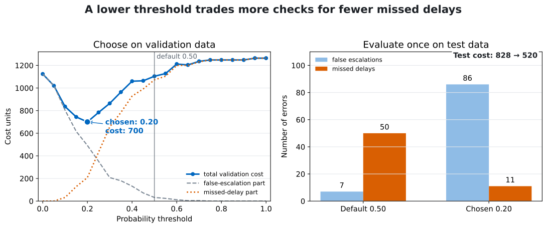
Read the left panel from low thresholds to high thresholds. The false-escalation part falls as fewer parcels are checked. The missed-delay part rises as more delayed parcels remain in the normal queue. Their sum reaches its lowest point at 0.20 for the stated costs.

Verify the rule once on test data

The chosen threshold must now be evaluated on rows that did not influence the choice. Calculate both the 0.50 rule and the selected 0.20 rule on the 240 test rows:

test = parcels.query("split == 'test'").copy()

test_default = threshold_metrics(test, 0.50)
test_chosen = threshold_metrics(test, chosen_threshold)

comparison = pd.DataFrame([
    {"rule": "default", **test_default},
    {"rule": "cost-sensitive", **test_chosen},
])

print(comparison[[
    "rule", "threshold", "true_positive", "false_positive",
    "false_negative", "true_negative", "accuracy", "recall",
    "total_cost",
]].round(3).to_string(index=False))

          rule  threshold  true_positive  false_positive  false_negative  true_negative  accuracy  recall  total_cost
       default        0.5             11               7              50            172     0.762    0.18         828
cost-sensitive        0.2             50              86              11             93     0.596    0.82         520

The selected threshold lowers test cost from 828 to 520 units, a reduction of about 37.2% under the fictional cost assumptions. It finds 50 of 61 delays instead of 11, so recall rises from 18.0% to 82.0%. The price is 79 additional false escalations.

Accuracy moves in the opposite direction, from 76.2% down to 59.6%. That is not a contradiction. Most parcels are not delayed, so a rule can obtain high accuracy by rarely escalating. Accuracy gives every mistake the same weight, while this decision says one missed delay costs four times as much as one unnecessary check.

Do not return to the test set to try 0.15, change the costs, and report whichever result looks best. That would make the test set another validation set. If the policy changes after this evaluation, use new labeled data for the next final check.

Check whether the cost choice changes the answer

Cost assumptions are often uncertain. A useful sensitivity check repeats the validation calculation with plausible values. It asks whether a different assumption would select a different rule.

Keep the false-escalation cost at 4 units and compare missed-delay costs of 8, 16, and 32 units. The next code still uses validation data only:

sensitivity_rows = []

for missed_cost in [8, 16, 32]:
    candidates = pd.DataFrame([
        threshold_metrics(
            validation,
            threshold,
            false_escalation_cost=4,
            missed_delay_cost=missed_cost,
        )
        for threshold in thresholds
    ])
    best = candidates.sort_values(
        ["total_cost", "threshold"]
    ).iloc[0]
    sensitivity_rows.append({
        "false_escalation_cost": 4,
        "missed_delay_cost": missed_cost,
        "chosen_threshold": best["threshold"],
        "validation_cost": int(best["total_cost"]),
    })

print(pd.DataFrame(sensitivity_rows).to_string(index=False))

 false_escalation_cost  missed_delay_cost  chosen_threshold  validation_cost
                     4                  8               0.3              536
                     4                 16               0.2              700
                     4                 32               0.1              868

When a missed delay costs only twice as much as an unnecessary check, the chosen threshold rises to 0.30. When it costs eight times as much, the threshold falls to 0.10. This result shows that a threshold is part of an operating policy. It is not a permanent property of the trained model.

Common mistakes and troubleshooting

Choosing the threshold on test data. Use validation data or cross-validation for selection, then evaluate once on untouched test data. The official scikit-learn threshold guide also warns against fitting a model and tuning its cutoff on the same rows because the decision rule can overfit those examples.

Treating 0.50 as a law. It is a common default, not a statement about your error costs, staffing capacity, or response time. Write down the action and its consequences before selecting a cutoff.

Using uncalibrated scores as probabilities. The cost workflow can compare score cutoffs, but a value such as 0.20 should only be described as a 20% chance when probability calibration has been checked. If that concept is new, read how to calibrate classifier probabilities in Python.

Reversing false positives and false negatives. Define the positive action in words first. Here, positive means “escalate as likely delayed.” A false positive is therefore an unnecessary escalation, while a false negative is a missed delay.

Leaving the boundary rule unclear. >= 0.20 includes a score of exactly 0.20; > 0.20 does not. Rounded probabilities can create many ties. Keep the comparison operator consistent in selection, evaluation, and production code.

Searching too narrow a range. Include thresholds that represent “act on every row” and “act on no rows,” or test every unique model score. A coarse grid is easy to teach but can miss a better cutoff between two steps.

Inventing precise costs without owners. The values 4 and 16 are fictional. In a real system, estimate time, money, service impact, or another agreed unit with people responsible for the decision. Run sensitivity checks when estimates are uncertain.

Ignoring capacity. A low-cost threshold may escalate more cases than a team can review. Add a capacity constraint or compare the top fixed number of cases instead of deploying an impossible rule.

Assuming the threshold never changes. Event rates, model calibration, process costs, and team capacity can change. Monitor them on new labeled data and repeat the documented selection process when the operating setting changes.

Recap

A classification model produces scores or estimated probabilities. A threshold turns those numbers into actions. The best candidate threshold for a policy depends on the consequences of false positives and false negatives, not only on a default value or the highest accuracy.

The practical workflow is:

1. Define the positive action and both error types.
2. Express their consequences in one consistent cost unit.
3. Compare candidate thresholds on validation data.
4. Document boundary and tie rules.
5. Select the lowest-cost valid threshold.
6. Evaluate it once on untouched test data.
7. Check whether reasonable cost changes would alter the decision.

For the fictional parcel data, the 0.20 validation choice reduced test cost from 828 to 520 units under the stated assumptions. Its accuracy was lower, but it found far more delays. The durable lesson is to optimize the decision you actually need, while keeping selection separate from final evaluation.