Compare LLM Prompts with a Paired Bootstrap in Python

Suppose you change an LLM prompt and its accuracy rises from 71.7% to 81.7%. The new prompt looks better, but the ten-percentage-point gap alone does not tell you how stable the improvement is. A different set of test cases could produce a smaller gap or even reverse it.

This tutorial compares two prompt versions on exactly the same maintenance notes. We will calculate their accuracy difference, keep each case paired during resampling, and report a 95% confidence interval. We will also inspect the cases on which only one prompt was correct.

The lesson uses saved predictions. It does not call an LLM API, so the results are reproducible and cost nothing to run. If you first need a basic evaluation harness, see how to evaluate local LLM tool routing. That tutorial focuses on labels and error analysis. This one focuses on comparing two versions with uncertainty.

Prerequisites and Setup

You need Python 3.10 or later and basic familiarity with a table. A pandas DataFrame is a table with named columns. NumPy handles numeric arrays, SciPy performs the resampling and test, and Matplotlib creates the chart.

Create and activate a virtual environment, then install the packages. On macOS or Linux, run:

python -m venv .venv
source .venv/bin/activate
python -m pip install numpy pandas scipy matplotlib

On Windows PowerShell, replace the activation command with .venv\Scripts\Activate.ps1.

The executed build used Python 3.13.2, NumPy 2.5.1, pandas 3.0.3, SciPy 1.18.0, and Matplotlib 3.11.0. Download the synthetic evaluation dataset and save it as maintenance_priority_evaluation.csv beside your Python file.

The dataset has 120 fictional equipment notes. It was generated for this tutorial and is released under CC0 1.0. It contains no real maintenance records and does not measure a real model. Each note has an expected priority—monitor, schedule, or urgent—plus saved predictions from Prompt A and Prompt B.

The Mental Model: Compare Each Case with Itself

Both prompts answer the same 120 cases. That detail makes the evaluation paired. Case M001 under Prompt A belongs with case M001 under Prompt B. The two results are not independent observations.

Imagine drawing a case ID from a container. When you draw M001, you take both prompt results for M001. You never take Prompt A’s M001 result and Prompt B’s M074 result. This keeps the note’s difficulty and wording fixed while you compare prompts.

A bootstrap repeats this sampling process many times with replacement. “With replacement” means a case can appear more than once in one resampled dataset, while another case may not appear. For each resample, we calculate:

Prompt B accuracy - Prompt A accuracy

The resulting collection of differences shows how much the measured improvement changes across resampled case mixes. We use the 2.5th and 97.5th percentiles of those differences as a 95% bootstrap confidence interval. The interval describes uncertainty in the estimated difference under this sampling method. It does not mean that 95% of future model answers will be correct.

Pairing matters because some notes are easy for both prompts and some are hard for both. Resampling each prompt separately would break that shared difficulty. SciPy’s current bootstrap documentation states that paired=True uses the same resampled indices for every input sample.

Load and Check the Evaluation Table

Start by reading the CSV. We print its shape and only the columns needed for the first comparison. This check catches wrong paths and unexpected schemas before any statistics are calculated.

import pandas as pd

evaluation = pd.read_csv("maintenance_priority_evaluation.csv")

print("shape:", evaluation.shape)
print(
    evaluation[
        ["case_id", "difficulty", "expected_priority",
         "prompt_a_prediction", "prompt_b_prediction"]
    ].head(5).to_string(index=False)
)

The executed output was:

shape: (120, 7)
case_id difficulty expected_priority prompt_a_prediction prompt_b_prediction
   M001       easy           monitor               monitor               monitor
   M002       easy          schedule              schedule              schedule
   M003       easy            urgent                urgent                urgent
   M004       easy           monitor               monitor               monitor
   M005       easy          schedule              schedule              schedule

Each row contains both predictions, so the pairing is explicit. Before comparing prompts, also check that every case ID occurs once and that no required value is missing:

required = [
    "case_id", "difficulty", "expected_priority",
    "prompt_a_prediction", "prompt_b_prediction",
]

assert evaluation["case_id"].is_unique
assert not evaluation[required].isna().any().any()
print("unique cases:", evaluation["case_id"].nunique())
print("missing required values:", int(evaluation[required].isna().sum().sum()))

unique cases: 120
missing required values: 0

These assertions stop the program if pairing is ambiguous. A duplicated case could give one note extra weight, while a missing prediction could silently change the sample used by one prompt.

Turn Predictions into Paired Correctness Values

Accuracy is the share of predictions equal to the expected label. Create one Boolean column for each prompt. A Boolean value is either True or False; pandas treats these as 1 and 0 when calculating a mean.

evaluation["a_correct"] = evaluation["prompt_a_prediction"].eq(
    evaluation["expected_priority"]
)
evaluation["b_correct"] = evaluation["prompt_b_prediction"].eq(
    evaluation["expected_priority"]
)

a_accuracy = evaluation["a_correct"].mean()
b_accuracy = evaluation["b_correct"].mean()
difference = b_accuracy - a_accuracy

print(f"Prompt A: {evaluation['a_correct'].sum()}/120 = {a_accuracy:.3f}")
print(f"Prompt B: {evaluation['b_correct'].sum()}/120 = {b_accuracy:.3f}")
print(f"B - A: {difference * 100:.1f} percentage points")

The executed result is:

Prompt A: 86/120 = 0.717
Prompt B: 98/120 = 0.817
B - A: 10.0 percentage points

A percentage point is the direct difference between two percentages. The change from 71.7% to 81.7% is 10.0 percentage points. Calling it a “10% increase” would be ambiguous because the relative increase is different.

Now split the result by difficulty. Grouping helps reveal whether the total improvement comes from only one part of the test set. pandas supports named output columns in GroupBy.agg, which keeps the summary readable.

by_difficulty = evaluation.groupby("difficulty", sort=False).agg(
    cases=("case_id", "size"),
    prompt_a_accuracy=("a_correct", "mean"),
    prompt_b_accuracy=("b_correct", "mean"),
)
print(by_difficulty.to_string(float_format=lambda value: f"{value:.2f}"))

            cases  prompt_a_accuracy  prompt_b_accuracy
difficulty
easy           40               0.90               0.95
medium         40               0.75               0.85
hard           40               0.50               0.65

Prompt B is higher in every difficulty group, while both prompts lose accuracy on harder notes. This is more informative than the overall score, but the sample still contains only 40 cases per group. We need an uncertainty estimate before treating each small group difference as stable.

Build a Paired Bootstrap Confidence Interval

SciPy expects a statistic function, which turns the two correctness arrays into the number we want to study. Our function returns Prompt B’s mean minus Prompt A’s mean. The axis argument lets SciPy calculate many resamples efficiently.

import numpy as np
from scipy.stats import bootstrap

def accuracy_difference(a, b, axis=-1):
    """Return Prompt B accuracy minus Prompt A accuracy."""
    return np.mean(b, axis=axis) - np.mean(a, axis=axis)

a = evaluation["a_correct"].to_numpy(dtype=float)
b = evaluation["b_correct"].to_numpy(dtype=float)

result = bootstrap(
    (a, b),
    accuracy_difference,
    paired=True,
    vectorized=True,
    n_resamples=20_000,
    method="percentile",
    rng=np.random.default_rng(20260714),
)

low = result.confidence_interval.low * 100
high = result.confidence_interval.high * 100
print(f"observed difference: {accuracy_difference(a, b) * 100:.1f} points")
print(f"95% paired bootstrap interval: {low:.1f} to {high:.1f} points")

The fixed random seed makes the teaching result repeatable. The executed output was:

observed difference: 10.0 points
95% paired bootstrap interval: 1.7 to 18.3 points

The full interval is above zero in this synthetic evaluation. That supports the limited conclusion that Prompt B performed better under this test design. The bootstrap procedure places the central 95% of resampled gains between 1.7 and 18.3 percentage points. It does not prove that Prompt B is better for every kind of request, language, model release, or production user.

The interval is also wide. The plausible improvement near its lower end is much smaller than the observed ten points. More representative cases would usually give a more useful estimate than simply increasing the number of resamples. Twenty thousand resamples cannot repair a narrow or biased test set.

The generated chart combines the difficulty results with the complete bootstrap distribution:

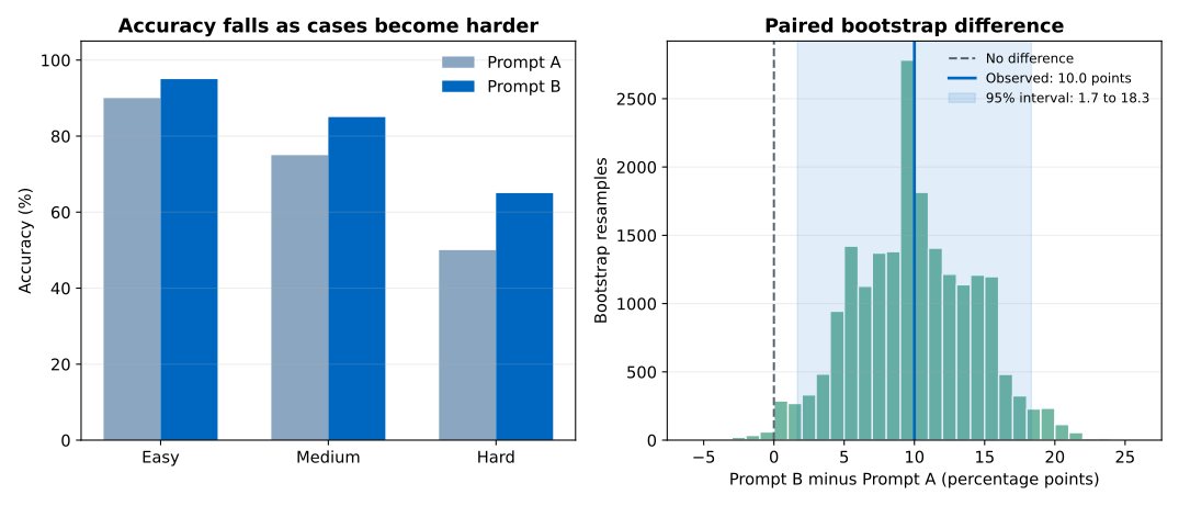
Read the left panel by comparing bars within each difficulty, not across unrelated datasets. Read the right panel against the dashed zero line. Most resamples fall to the right of zero, but their spread shows that the estimated gain changes with the selected cases.

Inspect Which Prompt Changed the Decision

Accuracy values hide the pairing details. Two prompts could have identical accuracy while succeeding on different cases. Count the four possible outcomes: both prompts correct, only A correct, only B correct, and neither prompt correct.

a_only = evaluation["a_correct"] & ~evaluation["b_correct"]
b_only = ~evaluation["a_correct"] & evaluation["b_correct"]

print("A only correct:", int(a_only.sum()))
print("B only correct:", int(b_only.sum()))
print("both correct:", int((evaluation["a_correct"] & evaluation["b_correct"]).sum()))
print("neither correct:", int((~evaluation["a_correct"] & ~evaluation["b_correct"]).sum()))

A only correct: 8
B only correct: 20
both correct: 78
neither correct: 14

Only the 28 disagreement cases affect the accuracy difference. Prompt B fixes 20 cases that A misses, but it also loses 8 cases that A gets right. This is why paired analysis is useful: it exposes both gains and regressions.

We can run an exact two-sided binomial test on those discordant cases. Under the null hypothesis that neither prompt has an advantage, each disagreement is equally likely to favor A or B. SciPy documents binomtest as a test of a success probability against a chosen value.

from scipy.stats import binomtest

discordant_count = int(a_only.sum() + b_only.sum())
test = binomtest(
    int(b_only.sum()),
    n=discordant_count,
    p=0.5,
    alternative="two-sided",
)
print(f"discordant cases: {discordant_count}")
print(f"exact two-sided p-value: {test.pvalue:.4f}")

discordant cases: 28
exact two-sided p-value: 0.0357

The p-value is the probability, under the equal-performance null model, of seeing an imbalance at least this strong in either direction. It is not the probability that Prompt B is better. The bootstrap interval is usually easier to use for decisions because it shows the estimated size and uncertainty of the gain. The exact test is a supporting check, not a replacement for reading failures.

Common Mistakes and Troubleshooting

You resample the two prompt columns independently. Use paired=True. Independent resampling destroys the case-by-case relationship and answers a different question.

The prompt versions use different test cases. A paired comparison requires the same cases and expected labels. Join results by a stable case ID, check uniqueness, and stop if either prediction is missing.

A higher score becomes a production claim. This dataset is synthetic and balanced by design. Repeat the evaluation on representative, reviewed cases from the intended task before making a deployment decision.

You tune prompts on the final evaluation set. Repeatedly reading failures and changing a prompt makes that set part of development. Keep a separate final test set that remains unseen until the prompt is fixed.

The confidence interval changes on every run. Pass a fixed NumPy generator through SciPy’s rng argument while developing. Record the seed and package versions. For a final analysis, confirm that reasonable seeds and resample counts do not change the practical conclusion.

The interval is narrow but the labels are weak. Statistical precision cannot correct unclear expected answers. Write a labeling guide, review ambiguous cases, and measure reviewer agreement for subjective tasks.

Accuracy hides costly errors. If an urgent note missed as monitor is more harmful than another error, report that failure separately or define a cost-sensitive metric before the comparison.

The SVG script fails on a server. Select Matplotlib’s Agg backend before importing matplotlib.pyplot. This headless backend writes files without opening a desktop window.

Recap

A prompt comparison starts with paired rows: one case, one expected answer, and one prediction from each prompt. Convert both predictions to correctness values, calculate Prompt B minus Prompt A, then resample case indices while keeping the pair together.

In this synthetic example, Prompt A scored 71.7% and Prompt B scored 81.7%. The observed gain was 10.0 percentage points, and the paired 95% bootstrap interval ran from 1.7 to 18.3 points. Prompt B alone was correct on 20 disagreement cases, while Prompt A alone was correct on 8.

The durable lesson is not “choose the prompt with the larger number.” It is: compare the same cases, show the size of the difference, report its uncertainty, and inspect every important regression. That combination gives you a result people can review and reproduce.