A maintenance assistant has three questions about a small rover: Is the battery safe, is the route clear, and is the radio link reliable? The useful facts live in a separate sequence of status records. Each question must select and combine the relevant source information.

To implement cross-attention in NumPy, place the requesting sequence in a query matrix and the source sequence in key and value matrices. Mask invalid source columns, calculate softmax(Q @ K.T / sqrt(d_k)), and multiply the weights by V; this produces one context row per query and one output feature per value column.

This lesson keeps every matrix small enough to inspect. We use hand-designed vectors instead of training a model, so the goal is to understand information flow and shapes. If the basic query-key-value calculation is new, first read scaled dot-product attention in NumPy.

Setup and the Two Synthetic Sequences

You need Python 3.11 or newer and basic knowledge of Python lists. A NumPy array is a rectangular collection of numbers. You do not need to know Transformer architecture or matrix algebra before starting; each operation is explained before it appears.

Create a virtual environment and install the packages used by the executed lesson:

python -m venv .venv
source .venv/bin/activate
python -m pip install numpy pandas matplotlib

On Windows PowerShell, activate the environment with .venv\Scripts\Activate.ps1. The executed results used Python 3.13.2, NumPy 2.5.1, pandas 3.0.3, and Matplotlib 3.11.0.

Download rover_questions.csv and rover_status_records.csv, then save both beside your Python file. These two original synthetic datasets were created for this lesson and are released under CC0-1.0. The rover, records, and numeric features are fictional; they are not measurements from a real machine.

The generated chart is an SVG file. Select Matplotlib’s headless Agg backend before importing pyplot so the same code works without a desktop display:

import matplotlib

matplotlib.use("Agg")

import matplotlib.pyplot as plt
import numpy as np
import pandas as pd

Load both files and print them before extracting arrays. The q_, k_, and v_ prefixes make each column’s role explicit:

questions = pd.read_csv("rover_questions.csv")
status_records = pd.read_csv("rover_status_records.csv")

print(questions.to_string(index=False))
print(status_records.to_string(index=False))

   question  q_energy  q_route  q_link
power check       2.2      0.1     0.0
route check       0.1      2.2     0.1
 link check       0.0      0.1     2.2
     record  k_energy  k_route  k_link  v_risk  v_readiness
battery low       2.2      0.2     0.0    0.95         0.15
route clear       0.1      2.2     0.1    0.10         0.95
 radio weak       0.0      0.2     2.2    0.80         0.35
 dock ready       1.5      0.6     0.1    0.15         1.00
      <pad>       0.0      0.0     0.0    0.00         0.00

Each question has three query features: energy, route, and link. Each source record has matching key features used for comparison. Its two value features carry the information that attention will mix: risk and readiness.

These features are teaching inputs, not text embeddings from a trained model. In a real network, learned projection layers usually create queries, keys, and values from earlier representations.

How Cross-Attention Works Between Two Sequences

An attention calculation gives the three matrix roles separate jobs:

• A query describes what one position wants to find.
• A key describes what each source position can match.
• A value contains the information that a matched source position contributes.

The word cross means the queries come from one sequence while the keys and values come from another. Here, three maintenance questions query five status positions. By contrast, self-attention takes queries, keys, and values from the same sequence.

Let T be the number of query positions, S the number of source positions, d_k the query-key width, and d_v the value width. The shapes in this lesson are:

queries Q:  (T, d_k) = (3, 3)
keys K:     (S, d_k) = (5, 3)
values V:   (S, d_v) = (5, 2)
weights:    (T, S)   = (3, 5)
context:    (T, d_v) = (3, 2)

The important result is rectangular. The weight matrix needs one cell for every query-source pair, so it has three rows and five columns. The context keeps the query length of three but takes its feature width of two from the values.

Scaled dot-product attention is written as:

attention(Q, K, V) = softmax(Q Kᵀ / sqrt(d_k)) V

The original Transformer paper gives this matrix form. It also distinguishes self-attention from the encoder-decoder attention in which queries read keys and values from another representation. We will use the same calculation for a domain-neutral teaching example rather than translation.

Build the Rectangular Score Map

First, select the columns by prefix and convert them to floating-point arrays. Print the shapes now; most attention errors become easier to locate when you know which axis is wrong:

queries = questions.filter(regex=r"^q_").to_numpy(float)
keys = status_records.filter(regex=r"^k_").to_numpy(float)
values = status_records.filter(regex=r"^v_").to_numpy(float)

print("queries:", queries.shape)
print("keys:", keys.shape)
print("values:", values.shape)

queries: (3, 3)
keys: (5, 3)
values: (5, 2)

Queries and keys share a width of three because their dot products compare matching features. Keys and values share a source length of five because every key must point to a value at the same source position. The value width can differ from the query-key width.

NumPy’s @ operator performs matrix multiplication. Transposing keys changes its shape from (5, 3) to (3, 5), so the product has shape (3, 5). Divide by the square root of the key width before softmax:

raw_scores = queries @ keys.T
scaled_scores = raw_scores / np.sqrt(keys.shape[1])

print("score shape:", scaled_scores.shape)
print(np.round(scaled_scores, 3))

score shape: (3, 5)
[[2.806 0.254 0.012 1.940 0.000]
 [0.381 2.806 0.381 0.854 0.000]
 [0.012 0.254 2.806 0.162 0.000]]

Read the first row as the power check query compared with all five source keys. Its largest score, 2.806, belongs to battery low. The dock ready record also receives a strong score of 1.940 because its key has a large energy feature.

For example, the first scaled score comes from this calculation:

((2.2 × 2.2) + (0.1 × 0.2) + (0.0 × 0.0)) / sqrt(3) = 2.806

The current NumPy matmul documentation describes the (n, k) @ (k, m) -> (n, m) shape rule used here. The division does not change the shape; it controls how score magnitude grows with query-key width.

Mask the Source and Normalize Each Query

<pad> is a placeholder used to make source sequences a common length. It is not a real status record. A zero key is not enough to hide it because a zero score still becomes exp(0), which is positive.

Create one Boolean per source position. Then replace the invalid score column with negative infinity before softmax:

valid_source = status_records["record"].ne("<pad>").to_numpy()

if not valid_source.any():
    raise ValueError("at least one source position must be valid")

masked_scores = np.where(
    valid_source[np.newaxis, :],
    scaled_scores,
    -np.inf,
)

print(valid_source)
print(masked_scores[:, -1])

[ True  True  True  True False]
[-inf -inf -inf]

The new axis expands the mask from shape (5,) to (1, 5). NumPy then broadcasts that row across all three queries. Cross-attention masks source columns because those columns identify the keys and values that queries may read.

Now define softmax, a function that turns each row into non-negative shares totaling 1. Subtracting the row maximum first prevents overflow without changing the final ratios:

def stable_softmax(scores):
    shifted = scores - scores.max(axis=-1, keepdims=True)
    exponentials = np.exp(shifted)
    return exponentials / exponentials.sum(axis=-1, keepdims=True)


weights = stable_softmax(masked_scores)
print(np.round(weights, 3))
print("row sums:", weights.sum(axis=1))
print("padding column:", weights[:, -1])

[[0.641 0.050 0.039 0.270 0.000]
 [0.067 0.758 0.067 0.108 0.000]
 [0.051 0.064 0.826 0.059 0.000]]
row sums: [1. 1. 1.]
padding column: [0. 0. 0.]

Each row is a separate distribution over the source. The power question takes 64.1% from battery low and 27.0% from dock ready. The route question takes 75.8% from route clear, while the link question takes 82.6% from radio weak. Padding receives no share.

NumPy’s exp reference confirms that exponentiation is element-wise. The subtraction, exponentiation, and division therefore act on every score, while axis=-1 keeps normalization within one query row.

Mix Source Values Into Context Vectors

Weights are intermediate results. The attention output comes from multiplying them by the values:

context = weights @ values

print("context shape:", context.shape)
print(np.round(context, 3))

context shape: (3, 2)
[[0.686 0.427]
 [0.209 0.861]
 [0.724 0.417]]

The rows still correspond to the power, route, and link questions. The columns now represent risk and readiness because those are the value features. The power context’s risk feature is the weighted sum of all source risk values:

0.641×0.95 + 0.050×0.10 + 0.039×0.80 + 0.270×0.15 + 0.000×0.00 ≈ 0.686

The route context has high readiness, 0.861, because it gives most of its weight to the route clear record, whose readiness value is 0.95, and some to dock ready, whose readiness value is 1.00. The link context has high risk, 0.724, because radio weak contributes most of that mixture. These meanings were designed into the teaching values; attention did not discover them through training.

The generated chart puts the weights and context side by side:

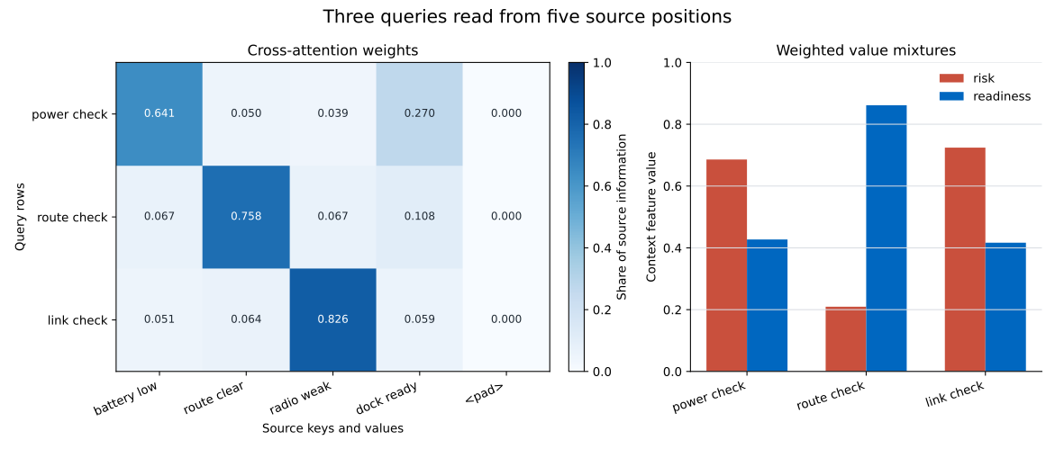
Read one heatmap row horizontally to see where one query collects information. Then find the same query in the bar chart to see the value mixture produced by those weights. The heatmap has five columns, but each context row has only two features because V has two columns.

Production APIs preserve this distinction. PyTorch’s scaled_dot_product_attention documentation names separate target length L, source length S, query-key width E, and value width Ev. Production tensors also add batch and attention-head axes, but the two-dimensional relationship shown here remains the core calculation.

Test Properties That Should Not Change

Looking at plausible numbers is not enough. Small tests can catch mask and alignment errors.

First, verify the two basic weight rules: every query row totals 1, and every padded source column is zero.

assert np.allclose(weights.sum(axis=1), 1.0)
assert np.all(weights[:, ~valid_source] == 0.0)

Next, put extreme values in the padded row and recalculate the context. A correct mask makes those values irrelevant:

extreme_values = values.copy()
extreme_values[-1] = [1_000_000.0, 1_000_000.0]
extreme_context = weights @ extreme_values

print(np.allclose(extreme_context, context))

True

This test is stronger than checking a normal zero padding value. It proves that the masked source cannot affect the result even when its value vector is large.

Keys and values also form aligned pairs. If you reorder source rows, apply the same order to keys, values, and the mask. The weight columns will move, but the context should stay the same:

order = np.array([2, 0, 3, 1, 4])
reordered_scores = queries @ keys[order].T / np.sqrt(keys.shape[1])
reordered_scores = np.where(valid_source[order][None, :], reordered_scores, -np.inf)
reordered_weights = stable_softmax(reordered_scores)
reordered_context = reordered_weights @ values[order]

print(np.allclose(reordered_context, context))

True

If you reorder keys but not values, a high match points to the wrong information. The shapes remain valid, so only a behavior test is likely to catch the error.

Common Mistakes and Troubleshooting

The matrix multiplication reports a width mismatch. The final width of queries must equal the final width of keys. Print both shapes. The values may use a different feature width.

Keys and values have different source lengths. Each key row identifies the value row at the same position. Require keys.shape[0] == values.shape[0] before calculating attention.

The mask is applied to query rows. A source padding mask belongs on the score columns. For one unbatched example, shape it as (1, source_length) so NumPy broadcasts it across queries.

Padding receives a small positive weight. Apply the mask before softmax. Zeroing weights afterward breaks the row total unless you normalize again.

Softmax produces nan. Subtract each row maximum before np.exp. Also reject a source in which every position is masked, as the earlier valid_source.any() check does. Softmax cannot create a valid distribution when there is nowhere to attend.

The context has the source length. The multiplication order should be (query_length, source_length) @ (source_length, value_width). The result follows query length, not source length.

A library mask uses the opposite convention. Mask meaning is API-specific. For example, PyTorch’s scaled dot-product function uses True for positions that participate, while nn.MultiheadAttention uses True in a key-padding mask for positions to ignore. Read the exact function’s documentation before moving this NumPy code into a framework.

Attention weights are treated as a full explanation. A weight shows how one attention operation mixed its value rows. It does not prove why an entire trained system made a final decision.

Recap: Follow the Query Length

Cross-attention lets one sequence read from another. The reusable shape rule is the easiest way to keep the calculation clear:

1. Queries supply the output rows.
2. Keys supply the source positions used for matching.
3. Values share the key length and supply the output features.
4. Q @ K.T creates a rectangular query-by-source score map.
5. A source mask blocks invalid columns before softmax.
6. weights @ V returns one context vector per query.

In the executed example, three questions attended to five status positions, producing a (3, 5) weight matrix and a (3, 2) context matrix. The lasting idea is simple: cross-attention may read a source of any length, but its output follows the query length and the value width.