Data Sampling for AI: A Practical Guide to Random, Stratified, and Systematic Sampling

Most datasets are too big, too slow, or too expensive to use in full. Maybe pulling every row means an API bill you don’t want to pay, maybe a model trains in minutes on a subset instead of hours on everything, or maybe the “full dataset” doesn’t even exist yet — you’re working with a snapshot of a population that’s still growing. So you sample: you pick a smaller set of rows and treat it as a stand-in for the whole. The question that decides whether that stand-in is any good isn’t “how big is my sample?” — it’s “does my sample actually look like the population it’s supposed to represent?”

That question is where people quietly go wrong. A sample can be large and still lie, and a sample can be tiny and still be honest. This is especially easy to get wrong once you’re feeding a sample into a machine learning model, because a biased sample doesn’t just skew a report — it teaches the model the wrong picture of reality, and it keeps doing that quietly until someone notices the model performs badly on exactly the group it under-saw during training. This guide builds one mental model for judging any sample, then works through the three sampling methods you’ll actually use — simple random, stratified, and systematic — on a real, imbalanced dataset, ending with why train_test_split is itself a sampling decision.

The Mental Model: Does Your Subset Lie?

Every sampling method is really just answering one question honestly, in three steps:

1. Name the population. What’s the full set of rows you’re trying to represent, and what does its breakdown look like on the column that matters — the one where getting the proportions wrong would actually hurt you?
2. Choose a method that gives every relevant subgroup a fair shot. Some methods (simple random) leave this to chance. Others (stratified) enforce it directly. Others (systematic) can accidentally violate it if the data has a hidden pattern.
3. Check the proportions, don’t assume them. Compare your sample’s breakdown on that same column to the population’s. If they don’t match, the method you picked didn’t do its job — no matter how “random” the process felt.

Step 3 is the one people skip. It’s tempting to assume that anything labeled “random” is automatically fair, but random and representative are not the same guarantee — you’ll see exactly how far apart they can be in a moment.

A Dataset You Can Reproduce

Say you’re prototyping a classifier that predicts whether a passenger would have survived a shipwreck, and the full dataset is inconvenient to work with on every iteration — you want a smaller working sample to iterate faster. Before you touch a model, you need to know whether that working sample still looks like the real thing.

We’ll use the titanic dataset — 891 passenger records with cabin class, sex, age, fare, and survival outcome — bundled with seaborn as a sample dataset.

import pandas as pd
import numpy as np
import seaborn as sns
from sklearn.model_selection import train_test_split

titanic = sns.load_dataset("titanic")
titanic.shape

(891, 15)

Data: the titanic dataset bundled with seaborn (seaborn.load_dataset), a widely used public teaching dataset compiled from the Kaggle Titanic competition and Encyclopedia Titanica passenger records — no download or account required beyond pip install seaborn.

titanic[["survived", "pclass", "class", "sex", "age", "fare"]].head()

   survived  pclass  class     sex   age     fare
0         0       3  Third    male  22.0   7.2500
1         1       1  First  female  38.0  71.2833
2         1       3  Third  female  26.0   7.9250
3         1       1  First  female  35.0  53.1000
4         0       3  Third    male  35.0   8.0500

891 rows, 15 columns. We’ll spend most of this post on class — First, Second, or Third — because it’s genuinely imbalanced, which is exactly what makes it useful for testing whether a sampling method is honest. (The outputs in this post come from pandas 3.0 and scikit-learn 1.9 — everything shown also works on pandas 2.x.)

titanic["class"].value_counts(normalize=True).round(3)

class
Third     0.551
First     0.242
Second    0.207
Name: proportion, dtype: float64

More than half of all passengers traveled Third class. If a sample of this dataset came back close to a 50/25/25 split, or worse, close to even thirds, you’d know something about how it was drawn went wrong.

Simple Random Sampling with .sample()

The most familiar method: every row gets an equal, independent chance of being picked. Pandas’ .sample() does exactly this.

sample = titanic.sample(n=90, random_state=3)
sample["class"].value_counts(normalize=True).round(3)

class
Third     0.600
First     0.233
Second    0.167
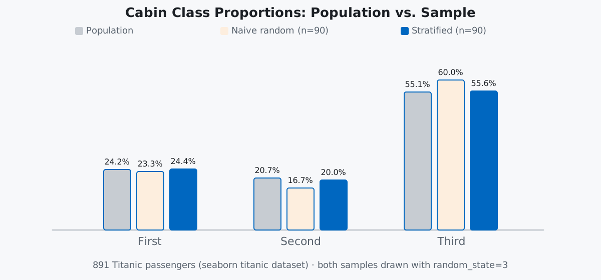
Name: proportion, dtype: float64

Read this against the population numbers above: Second class was 20.7% of the full dataset but only 16.7% of this sample, while Third class jumped from 55.1% to 60.0%. Nobody did anything wrong here — random_state=3 is just one honest, unlucky draw. That’s the catch with simple random sampling: it’s fair in expectation, not fair on any single run.

One Random Sample Isn’t Proof of Anything

To see how much a single draw can wobble, take five different random samples of the same size and watch the First-class share alone:

for seed in range(5):
    s = titanic.sample(n=90, random_state=seed)
    props = s["class"].value_counts(normalize=True).round(3)
    print(f"seed {seed}: First={props['First']}, Second={props['Second']}, Third={props['Third']}")

seed 0: First=0.333, Second=0.222, Third=0.444
seed 1: First=0.233, Second=0.244, Third=0.522
seed 2: First=0.222, Second=0.211, Third=0.567
seed 3: First=0.233, Second=0.167, Third=0.6
seed 4: First=0.144, Second=0.289, Third=0.567

The true First-class share is 24.2%. Across these five draws it ranges from 14.4% to 33.3% — more than a two-fold swing on the same population, the same sample size, and the same method. A single random sample is a coin flip on whether it happens to represent your minority groups well, and with a 90-row sample, class isn’t even your rarest possible category — imagine trying to sample a group that’s 2% of the population this way.

Stratified Sampling Preserves Proportions

Stratified sampling fixes this directly: split the population into groups (strata) first, then sample from each group in proportion to its size, instead of sampling from everyone at once. Pandas supports this natively through groupby().sample():

target_frac = 90 / len(titanic)
strat_sample = titanic.groupby("class", observed=True).sample(
    frac=target_frac, random_state=3
)
strat_sample["class"].value_counts(normalize=True).round(3)

class
Third     0.549
First     0.242
Second    0.209
Name: proportion, dtype: float64

Compare that to the population’s 55.1% / 24.2% / 20.7% — this is within a point of every group, every time, because each group was sampled on its own instead of leaving proportions to chance. Scikit-learn’s train_test_split offers the same guarantee through its stratify argument, which is the form you’ll use most often once you’re building a model rather than just exploring data:

strat_idx, _ = train_test_split(
    titanic.index, train_size=90, stratify=titanic["class"], random_state=3
)
strat_sample2 = titanic.loc[strat_idx]
strat_sample2["class"].value_counts(normalize=True).round(3)

class
Third     0.556
First     0.244
Second    0.200
Name: proportion, dtype: float64

Same idea, same result: 55.6% / 24.4% / 20.0%, again a close match. The trade-off is that stratified sampling needs you to already know which column matters enough to preserve — it can’t protect a category you didn’t think to stratify on.

Systematic Sampling: Every Nth Row

Systematic sampling takes every Nth row after picking a random starting point. It’s fast and simple, and on data in no particular order it can behave a lot like simple random sampling:

N = len(titanic) // 90  # step size for roughly 90 rows
systematic = titanic.iloc[::N]
systematic["class"].value_counts(normalize=True).round(3)

class
Third     0.586
Second    0.232
First     0.182
Name: proportion, dtype: float64

With a step of 9 on data in its original row order, this lands reasonably close to the population — not perfect, but not alarming either. The risk shows up the moment the data has any periodicity or grouping the step size can collide with. Watch what happens if the same dataset is sorted by class first — which is a completely ordinary thing to do before eyeballing a spreadsheet — and then sampled with a larger step:

sorted_titanic = titanic.sort_values("class").reset_index(drop=True)
trap_sample = sorted_titanic.iloc[::200]
trap_sample[["class"]].assign(row_index=trap_sample.index).reset_index(drop=True)

   class  row_index
0  First          0
1  First        200
2  Third        400
3  Third        600
4  Third        800

The sorted frame runs First (216 rows) then Second (184 rows) then Third (491 rows). A step of 200 jumps clean over the entire Second-class block — every single one of its 184 passengers has zero chance of being picked. This isn’t a contrived edge case; it’s what systematic sampling does by construction whenever the step size and the data’s ordering happen to line up. Only use systematic sampling on data you’re confident has no hidden structure, or shuffle it first.

Train/Test Split Is a Sampling Decision Too

Here’s the connection to AI specifically: when you call train_test_split, you’re not doing something separate from sampling — you’re sampling twice, once for the training set and once for the test set, from the same population. Everything above applies.

On the full 891-row dataset, splitting naively barely moves the needle, because the sample is large enough to average out:

X = titanic.drop(columns=["survived", "alive"])
y = titanic["survived"]
y.mean().round(3)  # population survival rate

X_train, X_test, y_train, y_test = train_test_split(X, y, test_size=0.2, random_state=3)
y_train.mean().round(3), y_test.mean().round(3)

population survived rate: 0.384
naive   train: 0.382  test: 0.391

But real projects rarely start with 891 clean rows — often you’re working with a smaller working sample, exactly like the one from the intro. Take a 150-row sample and split that naively:

small = titanic.sample(n=150, random_state=7)
X_small = small.drop(columns=["survived", "alive"])
y_small = small["survived"]
y_small.mean().round(3)  # 0.36

_, _, y_tr, y_te = train_test_split(X_small, y_small, test_size=0.3, random_state=0)
y_tr.mean().round(3), y_te.mean().round(3)

small-sample survived rate: 0.36
naive small       train: 0.324 (n= 105 ) test: 0.444 (n= 45 )

A training set where only 32.4% of examples survived, tested against a set where 44.4% did — a 12-point gap on a target that’s supposed to be the same 36% in both. A classifier trained on that split is learning a subtly wrong base rate, and you’d be evaluating it against a different one. Passing stratify=y_small fixes it the same way it fixed cabin class earlier:

_, _, y_tr_s, y_te_s = train_test_split(
    X_small, y_small, test_size=0.3, random_state=0, stratify=y_small
)
y_tr_s.mean().round(3), y_te_s.mean().round(3)

stratified small  train: 0.362 (n= 105 ) test: 0.356 (n= 45 )

Both land within half a point of the true 36% rate. This is exactly the same fix you’d reach for if your classes were more severely imbalanced than a roughly 60/40 split — fraud detection, rare-disease diagnosis, defect detection — where stratify= isn’t a nicety, it’s the difference between a training set that has seen enough of the minority class to learn anything about it and one that hasn’t.

Three Gotchas Worth Knowing

Sampling without a fixed seed makes your results irreproducible. Every .sample() call above passed random_state=. Drop it and you get a different sample on every run, which means a colleague — or you, next week — can’t check your work:

run1 = titanic.sample(n=5)["class"].tolist()
run2 = titanic.sample(n=5)["class"].tolist()
run1, run2

run 1: ['First', 'Third', 'Third', 'Third', 'Third']
run 2: ['Second', 'Third', 'Second', 'Third', 'Third']

Two calls, same code, two different results. Always pin random_state in anything you intend to rerun or hand off.

Sampling after a filter can quietly narrow your population without you noticing. Say you filter to adult_male passengers before sampling, because that’s the subgroup you’re analyzing today. The sample you draw afterward isn’t a sample of “passengers” anymore — it’s a sample of a population you’ve already reshaped:

adult_male_only = titanic[titanic["adult_male"]]
len(adult_male_only), len(titanic)
adult_male_only["class"].value_counts(normalize=True).round(3)

537 of 891 rows
class
Third     0.594
First     0.222
Second    0.184
Name: proportion, dtype: float64

537 rows is more than half the original dataset — it doesn’t feel small — but its class breakdown (59.4% Third) is already skewed away from the true population (55.1% Third) before any sampling method even runs. If you filter and then sample, be honest in your write-up about which population the sample actually represents.

A small sample and a biased sample are different problems, and fixing one doesn’t fix the other. The 90-row stratified samples earlier in this post are small — about 10% of the data — but their proportions were accurate to within a point. The 537-row adult_male filter above is large by comparison, but it’s still biased on class, because size was never the thing that was wrong. Before shrinking a sample or growing one, ask which problem you actually have.

Wrapping Up

Every sampling method answers the same question — does this subset look like the population? — with a different guarantee:

• Simple random (df.sample()) — fair in expectation, but any single draw can still misrepresent a category, especially with small samples or rare groups.
• Stratified (groupby().sample() or train_test_split(..., stratify=...)) — preserves known category proportions directly, at the cost of having to name the column that matters in advance.
• Systematic (df.iloc[::N]) — simple and fast on unordered data, but risks silently skipping entire groups if the data has any periodicity or grouping the step size collides with.
• Train/test split — not a separate step from sampling, but two samples drawn from the same population; use stratify= on your target column whenever it’s imbalanced.

If you want the foundations behind all of this — populations vs. samples, sampling error, and where these methods come from — the Statistics Fundamentals module in our free Statistics & Probability course covers exactly that. And once you’ve drawn a representative sample, Descriptive Statistics in Python shows you how to honestly describe what you’ve got.