A surface-inspection camera captures a tile with one pale, discolored area. A single average color for the whole image hides the problem, while a rule such as “red above 190” can fail when the lighting changes. A more useful question works at the pixel level: which pixels resemble the labeled defect examples?

To detect image defects with Gaussian Naive Bayes, convert every labeled pixel into a row of numeric color and texture features, keep complete images apart when splitting the data, fit GaussianNB, and reshape its pixel predictions into a mask—a grid that marks each pixel as clean or defective. Evaluate the mask on unseen images with defect precision, recall, and intersection over union; do not rely on pixel accuracy alone.

We will use twelve fictional tile images built for this lesson. The model learns from nine tiles and receives three complete tiles only during testing. This is a teaching workflow, not a real manufacturing specification.

Setup, Prerequisites, and Data

You need Python 3.11 or newer and basic knowledge of variables, arrays, and pandas tables. A classifier is a model that assigns a category to each example. Here, an example is one pixel, and the two categories are clean (0) and defect (1).

Create a virtual environment and install the packages used in the executed lesson:

python -m venv .venv
source .venv/bin/activate
python -m pip install numpy pandas scikit-learn scipy pillow matplotlib

On Windows PowerShell, activate it with .venv\Scripts\Activate.ps1. The published run used Python 3.13.2, NumPy 2.5.1, pandas 3.0.3, scikit-learn 1.9.0, SciPy 1.18.0, Pillow 12.3.0, and Matplotlib 3.11.0.

Download synthetic-tile-pixels.csv and save it beside your Python file or notebook. The 49,152-row dataset is original synthetic teaching data released under CC0-1.0. Its images, labels, colors, and defects are fictional. They do not describe a real material, camera, or quality limit.

The figure later in this tutorial is an SVG. To save it without opening a desktop window, select Matplotlib’s non-interactive Agg backend before importing pyplot. Then load the CSV and inspect a few rows before modeling:

import matplotlib

matplotlib.use("Agg")

import matplotlib.pyplot as plt
import numpy as np
import pandas as pd
from scipy.ndimage import binary_closing, binary_opening
from sklearn.metrics import confusion_matrix, jaccard_score, precision_score, recall_score
from sklearn.model_selection import GroupShuffleSplit
from sklearn.naive_bayes import GaussianNB

pixels = pd.read_csv("synthetic-tile-pixels.csv")
print(pixels.head(4).to_string(index=False))
print("shape:", pixels.shape)
print("tiles:", pixels["tile_id"].nunique())

tile_id  row  column  red  green  blue  red_minus_blue  green_minus_blue  local_contrast  is_defect
    T01    0       0  173    184   190           -17.0              -6.0          3.6356          0
    T01    0       1  181    188   199           -18.0             -11.0          3.4653          0
    T01    0       2  178    196   200           -22.0              -4.0          3.1285          0
    T01    0       3  177    189   191           -14.0              -2.0          2.4567          0
shape: (49152, 10)
tiles: 12

Each tile is 64 by 64 pixels, so it contributes 64 × 64 = 4,096 rows. The row and column fields preserve each pixel’s location. The target column, is_defect, contains the known label that the model should learn to predict.

Understanding Pixels as Classification Rows

Image segmentation means assigning a label to every pixel. The final result still looks like an image, but the classifier sees a table:

one image pixel -> one table row -> three features -> one predicted label

Raw red, green, and blue values can move together when a whole image becomes brighter. We instead use two color differences:

• red_minus_blue measures how much warmer a pixel is along the red-blue direction.
• green_minus_blue supplies a second color comparison.
• local_contrast measures brightness variation inside a 5 by 5 neighborhood.

A feature is an input column used for prediction. The first two features describe one pixel. The third adds limited information about nearby texture.

The dataset builder calculated local contrast as the brightness standard deviation within each neighborhood. This small version derives it from the neighborhood’s mean brightness and mean squared brightness for any RGB image stored as a NumPy array:

from scipy.ndimage import uniform_filter

rgb = image_array.astype(float)
brightness = rgb.mean(axis=2)
local_mean = uniform_filter(brightness, size=5, mode="reflect")
local_squared_mean = uniform_filter(brightness**2, size=5, mode="reflect")
local_contrast = np.sqrt(
    np.maximum(local_squared_mean - local_mean**2, 0)
)

feature_rows = np.column_stack([
    (rgb[:, :, 0] - rgb[:, :, 2]).ravel(),
    (rgb[:, :, 1] - rgb[:, :, 2]).ravel(),
    local_contrast.ravel(),
])
print(feature_rows.shape)

(4096, 3)

The ravel() calls flatten each 64 by 64 feature image into 4,096 values. np.column_stack places the three flattened arrays beside one another. Location is temporarily absent from the model inputs, but the row order lets us rebuild the mask later.

Gaussian Naive Bayes learns a bell-shaped, or Gaussian, distribution for every feature within every class. For a new pixel, it asks how compatible each feature value is with the clean and defect distributions. It combines that evidence with each class’s prior probability and selects the class with the larger score.

The word naive describes an assumption: after the class is known, the model treats the features as independent. Color differences and local contrast may not be truly independent. This simplification makes the model fast, but evaluation on separate images remains essential. The current scikit-learn Naive Bayes guide documents the Gaussian feature assumption and also warns that Naive Bayes probability estimates can be unreliable.

Hold Out Complete Images

Randomly splitting pixels would place neighboring pixels from one tile in both sets. Those pixels share lighting, base color, grain, and defect boundaries. A high test score could then measure similarity to the same image rather than performance on a new image.

Use tile_id as a group, which means a unit that must remain together. GroupShuffleSplit accepts group labels and produces row indices while keeping every group on one side. Its official API reference defines test_size in terms of groups rather than individual samples.

The next step reserves three entire tiles and keeps nine for training:

features = ["red_minus_blue", "green_minus_blue", "local_contrast"]

splitter = GroupShuffleSplit(
    n_splits=1,
    test_size=3,
    random_state=260722,
)
train_index, test_index = next(
    splitter.split(
        pixels[features],
        pixels["is_defect"],
        groups=pixels["tile_id"],
    )
)

train = pixels.iloc[train_index].copy()
test = pixels.iloc[test_index].copy()

print("train tiles:", sorted(train["tile_id"].unique()))
print("test tiles:", sorted(test["tile_id"].unique()))
print("shared tiles:", set(train["tile_id"]) & set(test["tile_id"]))
print("rows:", len(train), len(test))

train tiles: ['T01', 'T05', 'T06', 'T07', 'T08', 'T09', 'T10', 'T11', 'T12']
test tiles: ['T02', 'T03', 'T04']
shared tiles: set()
rows: 36864 12288

The empty set proves that no tile appears on both sides. random_state makes this particular group selection repeatable; it does not make the model more accurate.

Fit Gaussian Naive Bayes and Inspect What It Learned

Fit the model with the three feature columns and the training labels. Then print classes_ before selecting a probability column. This protects the code from assuming where the defect class appears:

model = GaussianNB()
model.fit(train[features], train["is_defect"])

learned_means = pd.DataFrame(
    model.theta_,
    index=model.classes_,
    columns=features,
)
print("class order:", model.classes_)
print("class priors:", model.class_prior_.round(3))
print(learned_means.round(2).to_string())

class order: [0 1]
class priors: [0.899 0.101]
   red_minus_blue  green_minus_blue  local_contrast
0          -21.00             -6.11            3.89
1           15.87              5.50            5.00

theta_ stores the learned mean of each feature for each class. Defect pixels are warmer in this designed dataset: their average red-minus-blue value is 15.87, compared with -21.00 for clean pixels. Their local contrast is also somewhat higher.

The priors show that about 10.1% of training pixels are defective. A prior is the class probability before the model sees the current features. It came from the training labels because we did not pass an explicit priors argument.

The values explain the fitted synthetic data; they are not reusable inspection thresholds. For a deeper look at how class priors combine with Gaussian evidence, see how to calculate Bayes error for Gaussian classes.

Turn Pixel Scores Back Into a Mask

predict_proba returns one column per class. Find the position of class 1, then use 0.5 as a simple demonstration threshold:

defect_column = np.flatnonzero(model.classes_ == 1)[0]
test["defect_probability"] = model.predict_proba(
    test[features]
)[:, defect_column]
test["prediction"] = (
    test["defect_probability"] >= 0.5
).astype(int)

tile = test.query("tile_id == 'T02'").sort_values(["row", "column"])
probability_mask = tile["defect_probability"].to_numpy().reshape(64, 64)
prediction_mask = tile["prediction"].to_numpy().reshape(64, 64)

print("probability shape:", probability_mask.shape)
print("predicted defect pixels:", prediction_mask.sum())

probability shape: (64, 64)
predicted defect pixels: 520

Sorting by row and column before reshape is important. The first 64 values become the first image row, the next 64 become the second row, and so on.

The probability map is useful for inspecting boundaries, but a pixel score of 0.8 must not be read as 80% physical certainty that the tile is defective. It is the model’s estimated probability for that pixel under its assumptions. Representative data and a separate calibration check are needed before treating such scores as reliable probabilities.

Measure the Mask, Not Just Pixel Accuracy

Most pixels are clean. A classifier that predicts “clean” for everything would score 86.9% accuracy on these test images while detecting no defective pixels. We therefore calculate three defect-focused measures:

• Precision is the share of predicted defect pixels that are truly defects.
• Recall is the share of true defect pixels that the model finds.
• Intersection over union (IoU) divides the overlap between predicted and known defect regions by their combined area.

Calculate all three on the untouched tiles. The confusion matrix uses actual classes as rows and predicted classes as columns:

y_test = test["is_defect"]
y_pred = test["prediction"]

print(f"all-clean accuracy: {(y_test == 0).mean():.3f}")
print(f"precision: {precision_score(y_test, y_pred):.3f}")
print(f"recall: {recall_score(y_test, y_pred):.3f}")
print(f"IoU: {jaccard_score(y_test, y_pred):.3f}")
print(confusion_matrix(y_test, y_pred, labels=[0, 1]))

all-clean accuracy: 0.869
precision: 1.000
recall: 0.975
IoU: 0.975
[[10682     0]
 [   40  1566]]

The model labels 1,566 defect pixels correctly and misses 40. It creates no false defect predictions in this designed test set, so precision is 1.000. The IoU of 0.975 shows strong region overlap.

These values are evidence about three unseen synthetic tiles under one deterministic design. They are not a benchmark for real camera images. Real surfaces can introduce glare, shadows, new pigments, scratches, label mistakes, and camera changes that are absent here.

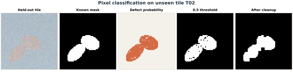
Read the panels from left to right. The probability map turns darker orange where the model finds stronger defect evidence. The threshold converts that continuous map into a binary mask: each pixel becomes either clean or defective. Comparing either predicted mask with the known mask reveals where the model misses the boundary.

Test Mask Cleanup Instead of Assuming It Helps

Pixel classifiers can produce isolated dots. Binary opening first erodes and then dilates a mask, which can remove objects smaller than the chosen neighborhood. Binary closing reverses that order and can fill small gaps. SciPy documents these operations in its current binary_opening reference.

Apply cleanup to each tile separately. Never reshape all test pixels into one combined image, because the edge of one tile would touch the next tile:

structure = np.ones((3, 3), dtype=bool)
cleaned_parts = []

for tile_id, rows in test.groupby("tile_id", sort=True):
    ordered = rows.sort_values(["row", "column"])
    raw_mask = ordered["prediction"].to_numpy().reshape(64, 64).astype(bool)
    cleaned_mask = binary_opening(raw_mask, structure=structure)
    cleaned_mask = binary_closing(cleaned_mask, structure=structure)
    cleaned_parts.append(pd.Series(cleaned_mask.ravel(), index=ordered.index))

test["cleaned_prediction"] = pd.concat(cleaned_parts).sort_index().astype(int)

cleaned = test["cleaned_prediction"]
print(f"cleaned precision: {precision_score(y_test, cleaned):.3f}")
print(f"cleaned recall: {recall_score(y_test, cleaned):.3f}")
print(f"cleaned IoU: {jaccard_score(y_test, cleaned):.3f}")
print(confusion_matrix(y_test, cleaned, labels=[0, 1]))

cleaned precision: 0.998
cleaned recall: 0.960
cleaned IoU: 0.958
[[10679     3]
 [   64  1542]]

Cleanup hurts this result. IoU falls from 0.975 to 0.958, and missed defect pixels increase from 40 to 64. The raw prediction contains no isolated false positives to remove, so erosion mainly removes correct boundary pixels. Keep the raw mask for this version of the workflow.

This comparison is why post-processing belongs inside evaluation. A technique that makes a mask look smoother can still make its measured overlap worse.

Common Mistakes and Troubleshooting

A random pixel split gives an unusually high score. Neighboring pixels from one image have shared conditions. Split with an image, patient, document, or scene identifier so complete groups stay apart.

The mask looks scrambled. Sort by row and column before reshaping. Also verify that every image contributes exactly height × width rows and that no rows were dropped during a merge.

The wrong probability column is used. Inspect model.classes_, then find the position of the desired label. Column 1 is not guaranteed to mean “defect” for every label type.

RGB and BGR are mixed. Pillow and Matplotlib commonly use RGB ordering. Some image libraries can use BGR. Confirm channel order before calculating color differences.

Morphological cleanup is chosen by appearance. Measure the raw and cleaned masks against untouched labels. Tune the structure size on validation images, not on the final test images.

Accuracy hides missed defects. Report the confusion matrix, precision, recall, and IoU for the class that matters. An all-clean baseline is a useful warning when defects are uncommon.

Probabilities are treated as calibrated confidence. Naive Bayes can return extreme probabilities when feature independence or Gaussian shapes are poor approximations. Check calibration separately before probabilities control an action.

Coordinates are added as features without a reason. Row and column help rebuild the mask, but using them for prediction can teach the model that defects occur in familiar positions. Include spatial features only when the position relationship is real and will remain stable.

Synthetic scores are used as deployment evidence. Replace this teaching data with representative labeled images. Document camera settings, sampling, label quality, allowed defect types, and the cost of each error. Re-test when any of those conditions change.

Recap: Keep the Image Boundary in the Workflow

The lasting idea is not only “one pixel becomes one row.” The image boundary must remain visible throughout the experiment:

• Derive numeric color or texture features for each pixel.
• Keep row and column only for rebuilding the mask unless location is a justified feature.
• Split by complete image so neighboring pixels cannot leak across the boundary.
• Fit GaussianNB and map probability columns through classes_.
• Reshape predictions in a verified row order.
• Compare masks with precision, recall, IoU, and confusion counts.
• Keep post-processing only when held-out evidence shows that it helps.

On the three unseen synthetic tiles, the raw mask reached 0.975 IoU with 40 missed defect pixels and no false defect pixels. A 3 by 3 opening-and-closing step looked smoother but reduced IoU to 0.958. That final result is a useful reminder: every extra image-processing step is a hypothesis to test, not a guaranteed improvement.

For a contrasting pixel workflow without labels, continue with finding dominant image colors using K-Means. That lesson treats pixels as rows too, but clustering discovers groups instead of learning from a known defect target.