A vibration sensor can drift as a machine warms, changes operating mode, and cools. Brief vibration peaks then occur at different baseline levels, so comparing raw readings can make short-lived changes harder to identify.

To detrend a nonlinear time series in Python, fit statsmodels LOWESS to time-ordered observations, keep the fitted values as the smooth trend, and subtract that trend from the observed values. Set return_sorted=False to align the fitted values with the original rows. Choose frac large enough to follow slow drift without also following the short events you want to preserve.

This tutorial applies that process to a fictional packaging-line sensor. The result is an additive residual in the original unit, millimetres per second (mm/s), so each remaining peak has a direct physical interpretation.

Before You Begin: Setup and Data

You should be able to run a Python file or a notebook cell. You do not need previous signal-processing or time-series experience. A time series is a set of observations ordered by time.

Create a virtual environment and install the four packages used here. On macOS or Linux, run:

python -m venv .venv
source .venv/bin/activate
python -m pip install numpy pandas matplotlib statsmodels

On Windows PowerShell, activate the environment with .venv\Scripts\Activate.ps1, then run the same pip install command. The executed build used Python 3.13.2, NumPy 2.5.1, pandas 3.0.3, Matplotlib 3.11.0, and statsmodels 0.14.6.

Download packaging_line_vibration.csv and save it beside your Python file. It contains 360 readings at two-minute intervals, covering 12 hours.

The dataset is original synthetic data generated with NumPy seed 20260728 and released under CC0-1.0. All measurements, times, equipment behavior, and vibration events are fictional. The simulation_drift_mm_s column records the drift used to construct the data. We will not use that column as an input to LOWESS; it exists only so we can verify span choices in this controlled lesson.

Select Matplotlib’s non-interactive Agg backend before importing pyplot. This lets the plotting code run on a server without a desktop display:

import matplotlib

matplotlib.use("Agg")

import matplotlib.pyplot as plt
import numpy as np
import pandas as pd
from statsmodels.nonparametric.smoothers_lowess import lowess

How LOWESS Detrending Works

We will describe every reading as two additive parts:

observed vibration = smooth trend + detrended residual

The trend is the slow-moving baseline. The residual is what remains after that baseline is removed. Detrending is therefore one subtraction:

detrended residual = observed vibration - smooth trend

LOWESS means locally weighted scatterplot smoothing. Instead of fitting one straight line across all 360 rows, it fits many small local lines. For each observation, nearby points receive more weight than distant points. The local estimates join to form a curve.

The main control is frac, a number between 0 and 1. It is the fraction of all observations used for each local estimate. With 360 rows:

frac=0.20 uses about 0.20 × 360 = 72 nearby observations
72 observations × 2 minutes = about 144 minutes of data

This 144-minute width is only an approximate interpretation for our evenly spaced readings. frac controls a fraction of the observed points, not a fixed clock duration.

A small frac creates a flexible curve. It may follow brief peaks and remove part of the signal that matters. A large frac makes a slower curve. It may miss a genuine bend in the baseline. The aim is not to make the residual as flat as possible. It is to separate changes that happen on different time scales.

Load the Readings and Check Their Order

Read the CSV, parse the timestamp strings as datetime values, and sort the rows. These checks come before smoothing because LOWESS needs an ordered numeric x-axis.

vibration = pd.read_csv(
    "packaging_line_vibration.csv",
    parse_dates=["timestamp"],
)
vibration = vibration.sort_values("timestamp").reset_index(drop=True)

print(vibration.head().to_string(index=False))
print("\nrows:", len(vibration))
print("frequency:", pd.infer_freq(vibration["timestamp"]))
print("duplicate timestamps:", vibration["timestamp"].duplicated().sum())
print("missing values:", vibration.isna().sum().sum())

The executed output is:

          timestamp  vibration_mm_s  simulation_drift_mm_s
2026-04-15 06:00:00          1.6156                 1.5506
2026-04-15 06:02:00          1.5893                 1.5554
2026-04-15 06:04:00          1.6098                 1.5601
2026-04-15 06:06:00          1.6660                 1.5647
2026-04-15 06:08:00          1.6398                 1.5692

rows: 360
frequency: 2min
duplicate timestamps: 0
missing values: 0

2min confirms that every adjacent row is two minutes apart. There are no duplicate times or missing values. Because the spacing is regular, a row number is a valid numeric representation of elapsed time for this fit.

If the timestamps were irregular, row number would incorrectly treat a two-minute gap and a two-hour gap as equal. In that case, create the x-axis from elapsed seconds:

elapsed_seconds = (
    vibration["timestamp"] - vibration["timestamp"].iloc[0]
).dt.total_seconds()

Do not fill an unknown sensor reading with zero unless the device truly measured zero. A fabricated zero can pull a local curve down. In the next section, missing="raise" makes LOWESS stop rather than silently dropping a row.

Fit the Curved Baseline and Subtract It

Start with frac=0.20, which uses about 72 neighboring readings. We also request three robust reweighting passes with it=3. These passes reduce the influence of observations with large residuals, so short peaks have less power to pull the baseline upward.

x = np.arange(len(vibration), dtype=float)

trend = lowess(
    endog=vibration["vibration_mm_s"].to_numpy(),
    exog=x,
    frac=0.20,
    it=3,
    is_sorted=True,
    missing="raise",
    return_sorted=False,
)

vibration["lowess_trend_mm_s"] = trend
vibration["residual_mm_s"] = (
    vibration["vibration_mm_s"] - vibration["lowess_trend_mm_s"]
)

The official statsmodels lowess documentation defines frac as the fraction of data used for each estimate. It also states that return_sorted=False returns fitted values in the input order. That alignment matters: using the default sorted, two-column result with an unsorted table could pair observations with the wrong fitted values.

Check the center and spread of the residuals. The median absolute deviation (MAD) measures a typical distance from the median and is less affected by large peaks than standard deviation.

residual_center = vibration["residual_mm_s"].median()
mad = (
    vibration["residual_mm_s"] - residual_center
).abs().median()
robust_sigma = 1.4826 * mad
review_threshold = residual_center + 4 * robust_sigma

flagged = vibration["residual_mm_s"] > review_threshold

reconstructed = (
    vibration["lowess_trend_mm_s"] + vibration["residual_mm_s"]
)
max_reconstruction_error = (
    vibration["vibration_mm_s"] - reconstructed
).abs().max()

print(f"selected frac: {0.20:.2f}")
print(f"residual median: {residual_center:.4f} mm/s")
print(f"robust sigma: {robust_sigma:.4f} mm/s")
print(f"review threshold: {review_threshold:.4f} mm/s")
print(f"flagged readings: {flagged.sum()}")
print(f"max reconstruction error: {max_reconstruction_error:.6f} mm/s")

The factor 1.4826 puts MAD on roughly the same scale as standard deviation when the ordinary noise is close to a normal distribution. The multiplier of four then creates a clear review rule. Neither value is a machine safety specification.

selected frac: 0.20
residual median: 0.0029 mm/s
robust sigma: 0.0638 mm/s
review threshold: 0.2583 mm/s
flagged readings: 24
max reconstruction error: 0.000000 mm/s

The residual median is close to zero, but that fact alone does not prove that the trend is correct. The 24 flagged rows are candidates for review, not confirmed faults. The zero reconstruction error checks the arithmetic: adding the trend and residual gives the original observation back.

Compare Three Smoothing Spans

The synthetic dataset gives us an advantage that real sensor data usually does not: we know the drift used during generation. We can fit three fractions and calculate mean absolute error (MAE) between each estimate and that known drift. Lower MAE means a closer match in this simulation.

span_records = []
fits = {}

for fraction in [0.08, 0.20, 0.45]:
    fitted = lowess(
        vibration["vibration_mm_s"].to_numpy(),
        x,
        frac=fraction,
        it=3,
        is_sorted=True,
        missing="raise",
        return_sorted=False,
    )
    fits[fraction] = fitted

    neighbors = int(np.ceil(fraction * len(vibration)))
    drift_mae = np.mean(
        np.abs(fitted - vibration["simulation_drift_mm_s"])
    )
    span_records.append({
        "frac": fraction,
        "approximate_neighbors": neighbors,
        "approximate_minutes": neighbors * 2,
        "drift_mae_mm_s": drift_mae,
    })

span_results = pd.DataFrame(span_records)
print(span_results.round({"drift_mae_mm_s": 4}).to_string(index=False))

 frac  approximate_neighbors  approximate_minutes  drift_mae_mm_s
 0.08                     29                   58          0.0353
 0.20                     72                  144          0.0133
 0.45                    162                  324          0.0178

The middle fraction has the lowest drift MAE, 0.0133 mm/s. The 0.08 curve is too responsive for this task: it follows some ordinary short-term movement and part of each peak. The 0.45 curve is slightly too rigid around bends in the baseline.

This comparison does not make 0.20 a universal setting. On real data, choose candidate spans from process knowledge. If drift takes several hours while events last ten minutes, test spans that sit between those scales. Then plot the results and check whether your conclusion changes under nearby values.

The downloadable lowess_span_results.csv contains the executed comparison.

Turn Flagged Rows into Reviewable Events

One vibration event can produce several consecutive flagged readings. Reviewing 24 separate rows would exaggerate the number of events, so group adjacent two-minute rows.

The next code starts a new group whenever the gap between flagged timestamps is greater than two minutes. cumsum() converts each new-group marker into an increasing event number.

flagged_rows = vibration.loc[
    flagged,
    ["timestamp", "vibration_mm_s", "residual_mm_s"],
].copy()

flagged_rows["new_group"] = (
    flagged_rows["timestamp"].diff() > pd.Timedelta("2min")
)
flagged_rows["excursion"] = flagged_rows["new_group"].cumsum() + 1

excursions = (
    flagged_rows.groupby("excursion", as_index=False)
    .agg(
        start=("timestamp", "min"),
        end=("timestamp", "max"),
        peak_residual_mm_s=("residual_mm_s", "max"),
        flagged_readings=("timestamp", "size"),
    )
)

print(
    excursions.round({"peak_residual_mm_s": 3}).to_string(index=False)
)

 excursion               start                 end  peak_residual_mm_s  flagged_readings
         1 2026-04-15 09:00:00 2026-04-15 09:16:00               0.750                 9
         2 2026-04-15 13:52:00 2026-04-15 14:20:00               1.006                15

The 24 readings reduce to two continuous groups. The second group lasts longer and reaches a larger residual peak of 1.006 mm/s. Because the baseline has been removed, that value means the observed vibration was about 1.006 mm/s above the local trend.

The threshold is a transparent screening rule for this lesson. It is not a safety limit and should not replace equipment specifications, maintenance records, or engineering review.

Plot the Trend, Residuals, and Span Check

The generated chart combines the important evidence. It compares the selected trend with the known synthetic drift, shows the residual threshold, and reports the three span errors.

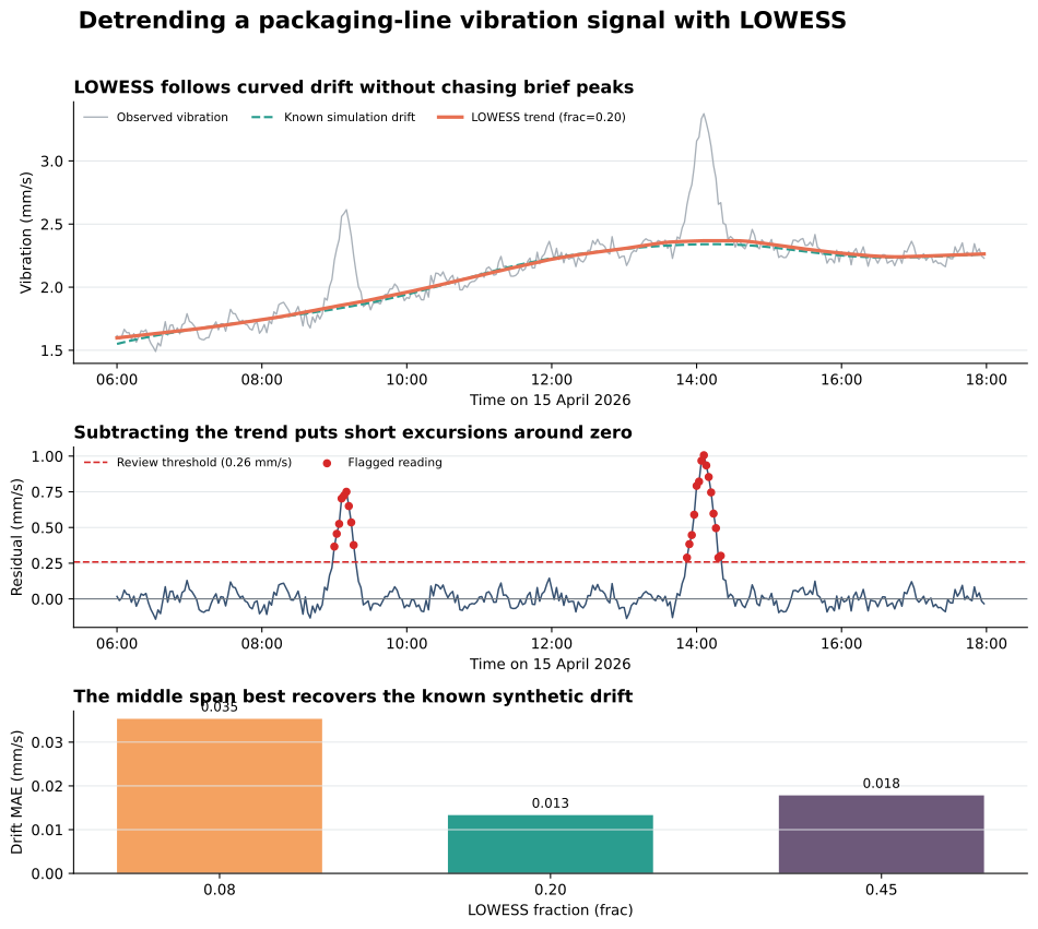
Read the top panel first. The orange LOWESS curve follows the slow green reference while leaving the two sharp peaks in the observations. In the middle panel, ordinary movement stays near zero, and both peaks cross the red review threshold. The bottom panel shows why the middle span was selected for this generated example.

If your goal is to separate a recurring calendar pattern after estimating a moving level, continue with weekly seasonality using pandas rolling windows. That tutorial answers a different question: it splits completed daily history into a baseline, weekday effect, and residual.

Common Mistakes and Troubleshooting

Treating frac as a fixed time window. It is a fraction of observations. The same frac covers a different duration when the row count or sampling interval changes. Convert it to an approximate number of points and minutes before interpreting it.

Using row number with irregular timestamps. LOWESS measures distance along exog. Use elapsed seconds when gaps vary, and decide how missing periods should affect the analysis.

Fitting unsorted data with is_sorted=True. This option promises that x is already increasing. Sort first, or leave is_sorted=False and manage the returned order carefully.

Letting a small span absorb the events. A very flexible trend can follow the peaks you wanted to study. Compare nearby spans and ask whether the fitted curve changes on the event time scale.

Using this centered smoother as a live forecast feature. A LOWESS value at an earlier row can depend on later neighbors. This is useful for analyzing completed history, but it can leak future information into forecasting or real-time alerting. Use a one-sided method for those tasks.

Trusting the first and last estimates equally. Points near the edges do not have neighbors on both sides. Inspect boundary values separately and avoid strong claims from a short edge segment.

Assuming detrending guarantees stationarity. A stationary series has statistical behavior that remains stable over time. Removing one smooth level may help, but changing variance, repeated cycles, and changing event rates can remain.

Using an additive residual when changes are proportional. Here, 0.5 mm/s above trend has the same meaning at every baseline. If variation grows with the signal level, a ratio or log-scale analysis may be more appropriate.

Recap and Where to Go Next

LOWESS detrending separates a slow nonlinear baseline from faster movement without requiring one global line. The durable workflow is:

1. Sort the time series and check timestamps, gaps, duplicates, and missing values.
2. Represent time with an increasing numeric x-axis.
3. Fit LOWESS with a span that is slower than the events of interest.
4. Keep fitted values in row order and subtract them from the observations.
5. Inspect residuals, boundaries, and nearby span choices before interpreting peaks.
6. Group consecutive flagged rows so one event does not look like many events.

For this synthetic signal, frac=0.20 used about 72 readings and recovered the known curved drift with 0.0133 mm/s MAE. Detrending then exposed two groups of high residuals. The important lesson is the separation of time scales, not the exact fraction or threshold.

For a real sensor, the next step is to compare residual events with maintenance logs and operating states. Keep the raw value, fitted trend, residual, chosen parameters, and timestamp together so another analyst can reproduce each alert and revise the baseline when the process changes.