How to Diagnose Neural Network Overfitting with Learning Curves

Epoch 420 is not the winner in this tutorial. Its training error is the lowest in the run, yet its predictions on unseen rows are worse than those from epoch 54. More training made the model fit its practice data better while performing worse on the real task.

A neural network is overfitting when training error continues to fall while validation error stops falling and begins to rise. Plot both errors by epoch, keep the model state with the lowest validation error, and leave the test set untouched until that choice is complete.

We will make that pattern visible with a small regression model. Regression means predicting a number. Here, the number is a fictional reading room’s energy use during the next hour.

Setup and prerequisites

You need Python 3.11 or newer. You should know basic Python variables and pandas tables, but you do not need to know neural-network mathematics. If train and test sets are new to you, start with How to Build Your First Machine Learning Model.

Create a virtual environment if you want to keep the lesson’s packages separate. Then install the four libraries used by the executed build:

python -m venv .venv
source .venv/bin/activate
python -m pip install numpy pandas scikit-learn matplotlib

On Windows PowerShell, activate the environment with .venv\Scripts\Activate.ps1. The published run used Python 3.13.2, NumPy 2.5.1, pandas 3.0.3, scikit-learn 1.9.0, and Matplotlib 3.11.0.

Download reading_room_energy.csv and save it beside your Python file. This is an original synthetic dataset generated with NumPy and random seed 84. Synthetic means code created the rows; they are not measurements from a real building. The 1,000 fictional observations are released under CC0-1.0.

Load the table and inspect a small set of columns before modeling. This check makes the row count, feature units, and numeric target visible:

import pandas as pd

energy = pd.read_csv("reading_room_energy.csv")
preview_columns = [
    "outside_temp_c",
    "visitors",
    "lighting_pct",
    "next_hour_kwh",
]

print(energy.shape)
print(energy[preview_columns].head(3).to_string(index=False))

(1000, 10)
 outside_temp_c  visitors  lighting_pct  next_hour_kwh
           24.6        22          64.2           9.58
           25.8        22          39.2           9.76
           27.9        17          60.5          11.70

There are 1,000 rows. next_hour_kwh is the target, measured in kilowatt-hours (kWh). The remaining numeric columns describe conditions such as temperature, visitor count, lighting, ventilation, sunlight, and hour-of-day position. The identifiers and all values are fictional, so the final error numbers are teaching results rather than evidence about real energy use.

Understanding what the two curves measure

A neural network changes its weights many times during training. One complete pass over the training rows is an epoch. After each epoch, we can ask two different questions:

1. How wrong is the model on rows that changed its weights?
2. How wrong is it on separate rows that did not change its weights?

The first answer is training error. The second is validation error. A learning curve plots either measurement against the number of epochs. Despite the name, it is not a list of learning-rate settings.

Both curves normally fall at first. The model is learning a pattern that works on known and unseen rows. Later, a flexible model can start fitting noise and details specific to the training sample. Training error keeps falling because those details help on the same rows. Validation error rises because they do not repeat elsewhere.

We will measure both curves with root mean squared error, or RMSE. It squares each error, averages the squares, and takes the square root. Lower is better, and the result returns to the target’s unit: kWh. Squaring means a few large misses have more influence than many small misses.

The important shape is not merely a gap between the curves. Validation error is often higher because the model has not trained on those rows. The stronger warning is a sustained direction change: training error keeps falling while validation error begins to rise.

Give training, validation, and test data separate jobs

We need three groups because they answer three different questions:

• Training rows update the model’s weights.
• Validation rows choose the epoch.
• Test rows measure the selected model once, after that choice.

First define the eight input features explicitly. Then reserve 30% of all rows as the final test set. Split the remaining rows again, keeping 220 for training and 480 for validation:

from sklearn.model_selection import train_test_split

feature_columns = [
    "outside_temp_c",
    "room_humidity_pct",
    "visitors",
    "lighting_pct",
    "ventilation_pct",
    "sunlight_w_m2",
    "hour_sin",
    "hour_cos",
]

X = energy[feature_columns]
y = energy["next_hour_kwh"]

X_development, X_test, y_development, y_test = train_test_split(
    X, y, test_size=0.30, random_state=84
)
X_train, X_validation, y_train, y_validation = train_test_split(
    X_development,
    y_development,
    train_size=220,
    random_state=84,
)

print("train:", X_train.shape)
print("validation:", X_validation.shape)
print("test:", X_test.shape)

train: (220, 8)
validation: (480, 8)
test: (300, 8)

The small training group is intentional. It makes a flexible network’s tendency to memorize easier to see. The validation group is larger, so its curve is less sensitive to one unusual row. The 300 test rows stay outside both training and epoch selection.

The features also have different scales. hour_sin stays between -1 and 1, while sunlight_w_m2 can be in the hundreds. Fit StandardScaler only on training rows, then apply those stored training statistics everywhere else:

from sklearn.preprocessing import StandardScaler

scaler = StandardScaler()
X_train_scaled = scaler.fit_transform(X_train)
X_validation_scaled = scaler.transform(X_validation)
X_test_scaled = scaler.transform(X_test)

fit_transform() learns a mean and standard deviation for every training feature. transform() reuses them without learning from validation or test rows. This follows scikit-learn’s data-leakage guidance: information used to prepare the model must not come from its final evaluation data.

Record one epoch at a time

The network has two hidden layers with 96 units each. This gives the model much more capacity than this small, clean training set requires, which makes overfitting easy to observe in a controlled example. alpha is also very small, so there is little penalty on large weights.

Create the regressor with a fixed random seed. The Adam solver adjusts weights from small batches of 32 rows:

from sklearn.neural_network import MLPRegressor

model = MLPRegressor(
    hidden_layer_sizes=(96, 96),
    activation="relu",
    solver="adam",
    alpha=0.000001,
    batch_size=32,
    learning_rate_init=0.002,
    shuffle=True,
    random_state=84,
)

scikit-learn’s current MLPRegressor reference defines partial_fit() as one iteration over the supplied data. Calling it in a loop lets us inspect both datasets after every epoch without updating the model from validation rows.

The next helper calculates RMSE. The loop also makes a deep copy whenever validation RMSE reaches a new minimum. A reference such as best_model = model would not be enough because later epochs would keep changing that same object.

import copy
import numpy as np
from sklearn.metrics import mean_squared_error

def rmse(actual, predicted):
    return np.sqrt(mean_squared_error(actual, predicted))

history = []
best_epoch = 0
best_validation_rmse = float("inf")
best_model = None

for epoch in range(1, 421):
    model.partial_fit(X_train_scaled, y_train)
    train_rmse = rmse(y_train, model.predict(X_train_scaled))
    validation_rmse = rmse(
        y_validation,
        model.predict(X_validation_scaled),
    )
    history.append((epoch, train_rmse, validation_rmse))

    if validation_rmse < best_validation_rmse:
        best_epoch = epoch
        best_validation_rmse = validation_rmse
        best_model = copy.deepcopy(model)

This long run is diagnostic. In a normal training job, an early-stopping rule would stop after a chosen number of epochs without meaningful validation improvement. Here, continuing to epoch 420 lets us see what that rule is preventing.

Convert the records to a DataFrame and print selected points from the run. The complete executed measurements are also available as learning_curve_metrics.csv.

curve = pd.DataFrame(
    history,
    columns=["epoch", "train_rmse_kwh", "validation_rmse_kwh"],
)
shown_epochs = [1, 20, 50, best_epoch, 100, 420]

print("best epoch:", best_epoch)
print(
    curve[curve["epoch"].isin(shown_epochs)]
    .round(3)
    .to_string(index=False)
)

best epoch: 54
 epoch  train_rmse_kwh  validation_rmse_kwh
     1          10.520               10.183
    20           1.705                2.052
    50           1.366                1.869
    54           1.336                1.867
   100           0.999                1.939
   420           0.243                2.427

At epoch 54, validation RMSE reaches its minimum of 1.867 kWh. Training RMSE then falls from 1.336 kWh to 0.243 kWh, but validation RMSE rises to 2.427 kWh. The final network fits the 220 training rows much more closely while producing worse predictions on the 480 validation rows.

Read the curves before choosing the model

The executed build saved this chart with Matplotlib’s headless Agg backend. The left panel shows the full run; the right panel enlarges the area around the validation minimum.

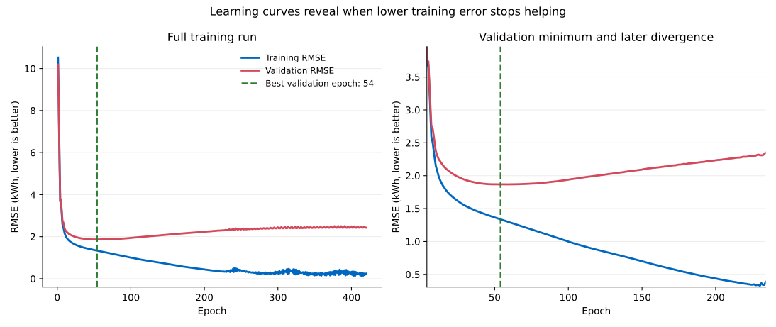
Read the blue training curve first. Its steady fall confirms that optimization is reducing error on the rows that update the weights. Now follow the red validation curve. It falls sharply, reaches its lowest point near epoch 54, then trends upward while the blue line continues downward.

That divergence is the evidence. Epoch 420 is not “more trained” in a generally useful sense. It is more specialized to this small training sample. Epoch 54 is the selected checkpoint because its validation error is lowest, not because 54 is a recommended number for other datasets.

The curve is not perfectly smooth. Mini-batch training and a finite validation sample create small changes from one epoch to the next. In a practical early-stopping rule, use patience: wait for several epochs without enough improvement before stopping. Patience avoids reacting to one small upward move, but it does not make the validation set independent. The validation set still influences model selection.

Test the selected checkpoint once

Only now should we use X_test_scaled. Compare the saved epoch-54 network with the epoch-420 network and a simple baseline that always predicts the mean of the training targets:

best_test_predictions = best_model.predict(X_test_scaled)
final_test_predictions = model.predict(X_test_scaled)
baseline_predictions = np.repeat(y_train.mean(), len(y_test))

print(f"epoch 54 test RMSE: {rmse(y_test, best_test_predictions):.3f} kWh")
print(f"epoch 420 test RMSE: {rmse(y_test, final_test_predictions):.3f} kWh")
print(f"mean baseline test RMSE: {rmse(y_test, baseline_predictions):.3f} kWh")

epoch 54 test RMSE: 1.871 kWh
epoch 420 test RMSE: 2.377 kWh
mean baseline test RMSE: 3.791 kWh

The validation-based choice also performs better on the untouched test data: epoch 54 has the lower test RMSE. It also beats the training-mean baseline. The final epoch still beats that simple baseline, but it is clearly worse than the saved checkpoint.

Do not choose epoch 54 because its test result looks good. The choice was already complete before generating any test predictions. If you inspect several checkpoints on test data and keep the best one, the test set quietly becomes another validation set. Its score will then be too optimistic as a final estimate.

Common mistakes and troubleshooting

Plotting training error alone. A falling training curve proves only that the network fits its training sample better. It cannot show whether performance on new rows is improving. Record validation error at the same epochs.

Using test rows to pick the stopping point. Keep a validation split for model choices. Use the test split after architecture, preprocessing, and epoch selection are fixed.

Fitting the scaler on all rows. That lets validation and test distributions affect training inputs. Split first, fit the scaler on X_train, and call only transform() on later groups.

Saving a reference instead of a checkpoint. best_model = model points to the object that continues training. Use copy.deepcopy() for this small in-memory lesson, or use a framework’s documented checkpoint mechanism for larger models.

Calling fit() repeatedly without checking its state rules. Some estimators reset parameters on each fit() call. This lesson uses partial_fit() because its documented action is one update iteration. Check the API of a different estimator before adapting the loop.

Stopping after the first worse epoch. Validation measurements can move slightly as mini-batch updates change the model. Use patience and a minimum improvement threshold. Save the best checkpoint seen during that waiting period.

Assuming every gap means overfitting. Validation error can be higher from the beginning because unseen rows are harder. Look for the training curve continuing downward while the validation curve reverses direction or remains worse for a sustained period.

Treating this synthetic score as a building forecast. The generator omits equipment changes, sensor failures, weather shifts, and human behavior. A real energy model needs representative data, time-aware evaluation when observations are ordered, domain review, and monitoring.

Recap and a useful next experiment

Learning curves turn overfitting from a vague warning into an observable pattern. Training data teaches the weights, validation data selects the checkpoint, and test data grades that completed choice.

The executed run made each role visible. Validation RMSE was lowest at epoch 54, at 1.867 kWh. By epoch 420, training RMSE had fallen to 0.243 kWh while validation RMSE had risen to 2.427 kWh. On untouched test rows, the saved checkpoint scored 1.871 kWh RMSE, compared with 2.377 kWh for the final network.

As a next experiment, change alpha from 0.000001 to 0.01 and rerun the same fixed splits. Plot the new curves beside the originals. A stronger weight penalty may narrow the train-validation gap, but compare the validation minimum rather than assuming that more regularization must help.