At 23:00, midnight is one hour away. In a raw hour column, however, 23 and 0 are the two most distant values. A linear model sees a jump of 23 units where the clock has a gap of only one hour.

To encode a cyclical time feature, convert each value to an angle over its known period, then add its sine and cosine as two model inputs. For hour-of-day, use angle = 2 * pi * hour / 24; this places 23:00 beside 00:00 on a circle while keeping every hour distinct. Fit and evaluate the complete model workflow on a split that matches how future predictions will be made.

This tutorial builds that representation, checks it by hand, and compares it with raw and one-hot hour inputs. The same idea applies to weekday, month, wind direction, and other features that repeat after a fixed period.

Setup and Prerequisites

You need Python 3.11 or newer and basic knowledge of table rows and columns. You should also know that a regression model predicts a number. No trigonometry or previous feature-engineering experience is required.

Create an isolated environment and install the four libraries used in the executed lesson:

python -m venv .venv
source .venv/bin/activate
python -m pip install numpy pandas scikit-learn matplotlib

On Windows PowerShell, activate the environment with .venv\Scripts\Activate.ps1. The published build used Python 3.13.2, NumPy 2.5.1, pandas 3.0.3, scikit-learn 1.9.0, and Matplotlib 3.11.0.

Download building_ventilation_readings.csv and save it beside your Python file. It is an original synthetic dataset released under CC0-1.0. Synthetic means code created the data. All 4,320 timestamps, temperatures, opening indicators, and power readings are fictional and do not describe a real building.

Each row contains one hourly observation from 1 January through 29 June 2025. The target, ventilation_power_kw, is fictional ventilation power in kilowatts. open_day is 1 when the building is open and 0 otherwise.

Load the CSV, parse its timestamp, and inspect a few rows before creating any model features:

import pandas as pd

readings = pd.read_csv(
    "building_ventilation_readings.csv",
    parse_dates=["recorded_at"],
)

print(readings.shape)
print(readings.head(4).to_string(index=False))

(4320, 5)
        recorded_at  hour  outdoor_temp_c  open_day  ventilation_power_kw
2025-01-01 00:00:00     0             6.7         1                  6.83
2025-01-01 01:00:00     1             5.6         1                  5.08
2025-01-01 02:00:00     2             5.5         1                  4.75
2025-01-01 03:00:00     3             7.7         1                  6.06

The first four rows cover midnight through 03:00. There are five published columns; the two cyclical columns will be derived next.

How Sine and Cosine Encoding Works

A cyclical feature repeats after a known period. The period is the number of steps in one complete cycle: 24 for hour-of-day and 7 for a weekday numbered from 0 through 6.

The raw hour values live on a line:

0 -- 1 -- 2 -- ... -- 22 -- 23

That line has no connection from 23 back to 0. We need a circle instead. Divide an hour by 24 to find its fraction of the day, multiply by 2 * pi to turn that fraction into an angle, then use two coordinates:

angle    = 2 * pi * hour / 24
hour_sin = sin(angle)
hour_cos = cos(angle)

Sine supplies the vertical coordinate and cosine supplies the horizontal coordinate. One coordinate alone is not enough because different hours can share the same sine or cosine value. Together, the pair identifies a position on the cycle.

The next function returns a new DataFrame with both coordinates. It does not estimate an average or another statistic from the dataset, so it has no fitted state:

import numpy as np

def add_cyclical_hour(data):
    valid_hour = (
        data["hour"].notna()
        & data["hour"].ge(0)
        & data["hour"].lt(24)
    )
    if not valid_hour.all():
        raise ValueError("hour must satisfy 0 <= hour < 24")

    angle = 2 * np.pi * data["hour"] / 24
    return data.assign(
        hour_sin=np.sin(angle),
        hour_cos=np.cos(angle),
    )


readings = add_cyclical_hour(readings)

NumPy’s current sin documentation expects angles in radians, where 2 * pi is one full turn. Inspect five points around the circle:

print(
    readings.loc[
        readings["hour"].isin([0, 6, 12, 18, 23]),
        ["hour", "hour_sin", "hour_cos"],
    ]
    .drop_duplicates()
    .sort_values("hour")
    .round(5)
    .to_string(index=False)
)

 hour  hour_sin  hour_cos
    0   0.00000   1.00000
    6   1.00000   0.00000
   12   0.00000  -1.00000
   18  -1.00000  -0.00000
   23  -0.25882   0.96593

Read the row for 00:00 as the point (cos=1, sin=0). At 06:00, the point has moved one quarter-turn. The value -0.00000 at 18:00 is ordinary floating-point rounding and is equal to zero for practical use.

Now check the boundary numerically. Euclidean distance is the straight-line distance between two coordinate pairs:

def cyclical_distance(first_hour, second_hour):
    hours = add_cyclical_hour(
        pd.DataFrame({"hour": [first_hour, second_hour]})
    )
    points = hours[["hour_sin", "hour_cos"]].to_numpy()
    return np.linalg.norm(points[0] - points[1])


print("raw distance, 23 to 0:", abs(23 - 0))
print("raw distance, 23 to 22:", abs(23 - 22))
print("cyclical distance, 23 to 0:", round(cyclical_distance(23, 0), 5))
print("cyclical distance, 23 to 22:", round(cyclical_distance(23, 22), 5))

raw distance, 23 to 0: 23
raw distance, 23 to 22: 1
cyclical distance, 23 to 0: 0.26105
cyclical distance, 23 to 22: 0.26105

The cyclical representation gives adjacent hours equal distance on both sides of 23:00. It also keeps distant hours apart: 12:00 lies on the opposite side of the circle from 00:00.

Hold Out the Future for Testing

The rows are ordered in time, so hold out the final 36 days. A chronological holdout trains on earlier rows and tests on later rows. This matches a workflow that uses past building readings to predict future readings.

The following split uses the first 144 complete days for training and the remaining 36 for testing:

split_at = 144 * 24
train = readings.iloc[:split_at].copy()
test = readings.iloc[split_at:].copy()

print("training:", len(train), train["recorded_at"].max())
print("test:    ", len(test), test["recorded_at"].min())

training: 3456 2025-05-24 23:00:00
test:     864 2025-05-25 00:00:00

The boundary is clean: the training data ends one hour before the test data begins. Randomly shuffling these rows would answer a different question because observations from the later period could enter the training set while earlier observations enter the test set.

This synthetic pattern is stable across the six months. Real building use may change because of holidays, operating schedules, equipment changes, or seasons. A time-aware split does not remove those changes; it reveals whether the workflow handles them.

Build Three Controlled Ridge Pipelines

We will compare three representations of the same hour:

1. Raw hour: one numeric column from 0 through 23.
2. One-hot hour: 24 binary columns, one for each possible hour.
3. Sine and cosine: two numeric columns that form a circle.

Every route also receives outdoor_temp_c and open_day. Every route uses the same Ridge regression model with alpha=1.0. Ridge is a linear regression model that limits very large coefficients. Keeping the model, rows, target, and non-time features fixed makes the hour representation the main experimental change.

Start with the raw route. StandardScaler learns the training mean and standard deviation, while ColumnTransformer sends named columns through that step:

from sklearn.compose import ColumnTransformer
from sklearn.linear_model import Ridge
from sklearn.pipeline import Pipeline
from sklearn.preprocessing import StandardScaler

raw_model = Pipeline([
    (
        "prepare",
        ColumnTransformer([
            (
                "numeric",
                StandardScaler(),
                ["hour", "outdoor_temp_c", "open_day"],
            )
        ]),
    ),
    ("model", Ridge(alpha=1.0)),
])

The one-hot route handles hour as a category. The 24 categories are declared explicitly, so the transformed shape stays consistent even if a smaller training sample is missing one hour:

from sklearn.preprocessing import OneHotEncoder

one_hot_model = Pipeline([
    (
        "prepare",
        ColumnTransformer([
            (
                "hour",
                OneHotEncoder(
                    categories=[list(range(24))],
                    handle_unknown="ignore",
                    sparse_output=False,
                ),
                ["hour"],
            ),
            (
                "numeric",
                StandardScaler(),
                ["outdoor_temp_c", "open_day"],
            ),
        ]),
    ),
    ("model", Ridge(alpha=1.0)),
])

OneHotEncoder creates one binary feature for each declared category. Its official API reference explains the categories, handle_unknown, and sparse_output options.

The cyclical route needs only the two new coordinates plus the other numeric features:

cyclical_model = Pipeline([
    (
        "prepare",
        ColumnTransformer([
            (
                "numeric",
                StandardScaler(),
                [
                    "hour_sin",
                    "hour_cos",
                    "outdoor_temp_c",
                    "open_day",
                ],
            )
        ]),
    ),
    ("model", Ridge(alpha=1.0)),
])

All scaling remains inside each pipeline. Calling .fit() on a pipeline calculates scaling statistics from train only, then fits Ridge on those transformed training rows. If this split-first rule is new, Preparing Data for Machine Learning in scikit-learn explains why every learned preprocessing step belongs inside the training workflow.

Compare Error and Feature Count

Fit each complete pipeline, predict the same test rows, and calculate two error measures. Mean absolute error (MAE) is the average absolute difference between prediction and target. Root mean squared error (RMSE) gives larger mistakes more weight. Lower is better for both, and both remain in kilowatts.

The feature map keeps the cyclical model from receiving the raw hour:

from sklearn.metrics import mean_absolute_error, root_mean_squared_error

models = {
    "Raw hour": raw_model,
    "One-hot hour": one_hot_model,
    "Sine + cosine": cyclical_model,
}
feature_columns = {
    "Raw hour": ["hour", "outdoor_temp_c", "open_day"],
    "One-hot hour": ["hour", "outdoor_temp_c", "open_day"],
    "Sine + cosine": [
        "hour_sin",
        "hour_cos",
        "outdoor_temp_c",
        "open_day",
    ],
}

rows = []
predictions = {}

for name, model in models.items():
    columns = feature_columns[name]
    model.fit(train[columns], train["ventilation_power_kw"])
    prediction = model.predict(test[columns])
    predictions[name] = prediction

    transformed = model.named_steps["prepare"].transform(
        train[columns].iloc[:1]
    )
    rows.append({
        "method": name,
        "transformed_features": transformed.shape[1],
        "test_mae_kw": mean_absolute_error(
            test["ventilation_power_kw"],
            prediction,
        ),
        "test_rmse_kw": root_mean_squared_error(
            test["ventilation_power_kw"],
            prediction,
        ),
    })

comparison = pd.DataFrame(rows)
print(comparison.round(4).to_string(index=False))

       method  transformed_features  test_mae_kw  test_rmse_kw
     Raw hour                     3       1.8529        2.2631
 One-hot hour                    26       0.7007        0.8652
Sine + cosine                     4       0.6985        0.8624

The raw-hour model has 1.853 kW MAE. Its one coefficient for hour can describe only a straight rising or falling trend, not a daily curve that returns to its starting point.

Both alternative representations reduce MAE to about 0.70 kW on the same 864 test rows. One-hot encoding uses 24 hour columns plus temperature and opening status, for 26 features. Sine and cosine reach a slightly lower error with four total features. The difference between 0.7007 and 0.6985 kW is small; this single synthetic holdout does not establish a universal winner.

You can inspect the exact executed metrics in cyclical_encoding_model_results.csv.

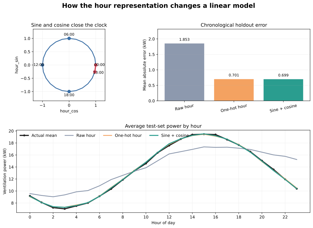
Read the lower panel from left to right. The raw-hour line cannot turn with the daily pattern. One-hot hour can learn a separate level at every hour, while sine and cosine produce one smooth cycle. This dataset was designed with a smooth daily relationship, so the compact cyclic representation matches it well.

Scikit-learn’s current time-related feature-engineering example makes an important broader point: one-hot, trigonometric, periodic spline, and tree-based routes have different flexibility. Sine and cosine remove the end-of-cycle jump, but one pair cannot describe every possible multi-peak pattern.

Inspect the Midnight Boundary Directly

Average metrics can hide one sharp discontinuity. Create two otherwise identical rows for 23:00 and 00:00, then ask each fitted model for a prediction:

boundary = pd.DataFrame({
    "hour": [23, 0],
    "outdoor_temp_c": [18.0, 18.0],
    "open_day": [1, 1],
})
boundary = add_cyclical_hour(boundary)

for name, model in models.items():
    columns = feature_columns[name]
    values = model.predict(boundary[columns])
    print(name, values.round(3))

Raw hour [16.494 11.45 ]
One-hot hour [11.523 10.381]
Sine + cosine [11.433 10.444]

The raw model drops by about 5.04 kW when the clock moves one hour. The one-hot and cyclical models change by about 1.14 and 0.99 kW. The cyclic model’s prediction is not forced to be identical at 23:00 and 00:00; those are neighboring points, not the same point.

This test holds temperature and opening status constant, so it isolates the hour representation. It is a useful check whenever a prediction curve should cross a boundary smoothly.

Choose the Representation That Matches the Feature

Use sine and cosine when the period is known, the boundary should be continuous, and a smooth relationship is plausible. Common examples include:

• hour-of-day with period 24;
• weekday numbered 0 through 6 with period 7;
• month numbered 1 through 12 with period 12;
• compass direction in degrees with period 360.

One-hot encoding can be a better first choice when the cycle has a small number of levels and neighboring levels may differ sharply. It lets a linear model estimate each hour independently, but it uses more columns and does not tell the model that 23:00 and 00:00 are neighbors.

A single sine-cosine pair describes one smooth wave. If demand has separate sharp morning and evening peaks, try higher-frequency sine-cosine pairs, periodic splines, or a model that can learn nonlinear shapes. Compare complete workflows on protected validation data rather than choosing from the training fit.

Tree models can often learn useful splits from a raw integer hour because they do not require one global straight-line coefficient. Cyclical encoding may still help, but it is not automatic. Test both routes with the same evaluation plan.

The related two-head PyTorch tutorial uses hour_sin and hour_cos as inputs to a neural network. This lesson supplies the boundary reasoning and controlled comparison behind those two columns.

Common Mistakes and Troubleshooting

Using 23 as the hourly period. There are 24 positions in a day, from 0 through 23. Divide by 24. Dividing by 23 maps hour 23 onto the same point as hour 0 even though they are different clock positions.

Creating only a sine column. Sine repeats values within one cycle. For example, different hours can have the same vertical coordinate. Keep both sine and cosine so the model receives a unique two-dimensional position.

Passing degrees directly to NumPy. np.sin() and np.cos() expect radians. Convert a cycle fraction with 2 * np.pi * value / period.

Encoding a feature that does not truly wrap. Age, income, and elapsed duration do not return to their starting value at a maximum. Do not encode them as circles. A feature is cyclical only when its end and start are genuine neighbors.

Ignoring invalid values. Check that each hour satisfies 0 <= hour < 24 before encoding it, as add_cyclical_hour() does above. The formula would otherwise wrap hour 24 onto hour 0 and could hide an upstream timestamp error.

Using the wrong local time. Hour-of-day usually describes local behavior. Convert timestamps to the intended timezone before extracting the hour, and decide how repeated or missing clock times during daylight-saving changes should be handled.

Shuffling time-ordered evaluation rows. If the final application predicts later periods, keep later rows after earlier rows. A random split can hide seasonal or operational change.

Assuming lower error proves a general rule. These measurements come from one controlled synthetic dataset. Repeat the comparison on representative validation periods from your own problem, and inspect boundary predictions as well as average error.

Recap and Next Step

A clock does not belong on a straight number line. Convert a cyclical value to an angle, then keep its sine and cosine coordinates. That makes the last and first positions neighbors without collapsing them into the same value.

In the executed building-ventilation comparison, raw hour produced 1.8529 kW test MAE. One-hot hour reduced it to 0.7007 kW with 26 transformed features. Sine and cosine used four total features and reached 0.6985 kW. Those results support the chosen representation for this smooth synthetic cycle, not for every dataset.

For your own data, write down the true period, validate the input range, create both coordinates, and use a split that matches future prediction. Then compare raw, one-hot, cyclic, and more flexible routes with the same model and rows. The reliable habit is to make the feature’s geometry match its real meaning, then verify the choice with held-out evidence.