How to Analyze Your Facebook Posting History with Python

“Am I posting too much?” isn’t a feeling — it’s a rate question, and Facebook will hand you the raw material to answer it. Every account can download its own post history as JSON through Settings → Your Facebook Information → Download Your Information, with a timestamp and the actual text of every post you’ve made. Most people download it once, skim a few entries, and never open the file again, because a nested JSON blob doesn’t look like an answer.

That’s where this project picks up, and it’s the same idea behind our Netflix viewing history project — turning your own platform export into real numbers instead of a vague impression — just applied to a different platform with a genuinely different data shape. A Netflix export is a flat two-column log of titles and dates; a Facebook export nests the post text inside a JSON structure and needs real time-zone handling before the dates mean anything. If you haven’t worked with Python’s date tools before, our Python datetime guide covers the fundamentals this project leans on. Below, we build a small mental model for “posting too much” first, then work through it hands-on on a sample file shaped exactly like your real export.

To find out if you post too much on Facebook, load your JSON export into pandas, convert its Unix-timestamp field into real datetimes in your own time zone, count posts per calendar day — including the days with zero posts — and compare that daily rate against your busiest outlier days. A day sitting several times above your average, not just “a lot of posts,” is what actually earns the label “too much.”

The Mental Model: Bucket, Rate, Compare

A posting history is really just a list of timestamps. “Do I post too much” isn’t a question about any single post — it’s a question about how dense those timestamps get in some window of time. Every version of that question routes through the same three moves:

1. Bucket every timestamp into a fixed window — a calendar day here, though the same idea works for a week or an hour.
2. Rate the buckets by turning each one’s raw count into a number you can compare, which only works if every bucket is represented, including the ones with zero posts.
3. Compare each bucket’s rate against a baseline — usually the overall average — to see which windows are unusually dense. That comparison, not the raw count, is the actual answer.

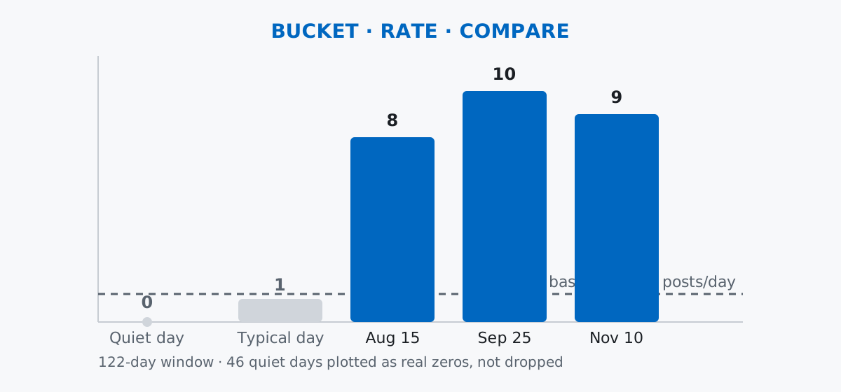
Notice the quiet day in that chart is plotted as an honest zero, not skipped. Skipping it is the single most common mistake in this kind of analysis, and it inflates your rate — we’ll hit it directly in a moment.

A Dataset You Can Reproduce (Shaped Like Facebook’s Own Export)

Facebook’s real export nests each post inside a data list, because the same structure has to describe photo posts, check-ins, and text posts with one schema — a post’s text lives at data[0]["post"], but photo-only posts have no post key at all. The top-level timestamp field is Unix epoch seconds in UTC, regardless of where you actually posted from.

That file is inherently personal, so there’s nothing real to vendor here. Instead, generate a synthetic file with the same shape and the same quirks for a clearly fictional persona, seeded so your numbers match this post exactly. Imagine Marta, who runs a small home-bakery Facebook page called Ferment & Flour and posts about her bakes over four months:

import json
import numpy as np
import pandas as pd
from datetime import datetime, timezone

rng = np.random.default_rng(42)

start = datetime(2025, 8, 1, tzinfo=timezone.utc)
n_days = 122  # 2025-08-01 through 2025-11-30

# Most days: 0, 1, or 2 posts (Poisson baseline). A few days get a deliberate
# burst added on top -- the "bake sale went viral" days.
daily_counts = rng.poisson(0.9, size=n_days)
burst_days = {14: 9, 55: 12, 101: 7}
for day_idx, extra in burst_days.items():
    daily_counts[day_idx] += extra

normal_posts = [
    "Tried a new sourdough starter this morning, smells incredible so far.",
    "Quiet baking day, just restocking the freezer with dough balls.",
    "Cinnamon rolls proofing on the counter, patience is the hard part.",
    "Swapped the usual flour blend for a rye mix today, texture is different.",
    "Cleaned out the pantry and found three bags of forgotten walnuts.",
    "Slow morning, one loaf in the oven and coffee in hand.",
    "Testing a new hydration ratio on the weekend batch.",
    "Grateful for the regulars who stop by every Thursday.",
]
link_posts = [
    "New recipe write-up is live, full method and timing here: https://example-bakery-notes.test/sourdough-timing",
    "Wrote up the whole bake-sale weekend, photos and numbers: https://example-bakery-notes.test/bake-sale-recap",
    "Sharing my starter-feeding schedule as a downloadable sheet: https://example-bakery-notes.test/starter-schedule",
]
caps_posts = [
    "SOLD OUT IN UNDER AN HOUR THANK YOU EVERYONE",
    "LAST CALL FOR SATURDAY PRE ORDERS CLOSES TONIGHT",
    "WE HIT ONE HUNDRED LOAVES THIS MONTH",
]
excited_posts = [
    "Back from the farmers market with the best strawberries!!!",
    "The oven finally arrived and it is even bigger than I hoped!!",
    "First sourdough discard crackers came out perfect!!!",
]

def make_text(rng):
    roll = rng.random()
    if roll < 0.10:
        return rng.choice(link_posts)
    if roll < 0.18:
        return rng.choice(caps_posts)
    if roll < 0.30:
        return rng.choice(excited_posts)
    return rng.choice(normal_posts)

records = []
for day_idx in range(n_days):
    count = int(daily_counts[day_idx])
    day_start = start + pd.Timedelta(days=day_idx)
    for _ in range(count):
        hour = int(rng.integers(6, 24))
        minute = int(rng.integers(0, 60))
        second = int(rng.integers(0, 60))
        ts = day_start.replace(hour=hour, minute=minute, second=second)
        unix_ts = int(ts.timestamp())

        # ~12% of posts are photo/album posts with no "post" text key --
        # a real quirk of Facebook's export, not a data-quality bug.
        if rng.random() < 0.12:
            data = [{"media_map": {"0": {"uri": "photos_and_videos/mock.jpg"}}}]
        else:
            data = [{"post": make_text(rng)}]

        records.append({"timestamp": unix_ts, "data": data})

export = {"status_updates_v2": records}
with open("your_posts.json", "w", encoding="utf-8") as f:
    json.dump(export, f, ensure_ascii=False)

len(records)

139

Data: a synthetic file (no license — generated for this post) shaped like Facebook’s real your_posts_1.json export from Download Your Information. (The outputs in this post come from pandas 3.0 — everything shown also works on pandas 2.x.)

Loading and Flattening the Export

Read the JSON back the way you’d read your own download. The top-level key is status_updates_v2, and each record’s data field is still a list of dictionaries — pandas won’t unpack it for you:

with open("your_posts.json", "r", encoding="utf-8") as f:
    raw = json.load(f)

posts = pd.DataFrame(raw["status_updates_v2"])
posts.head()

    timestamp                                               data
0  1754037310  [{'post': 'Grateful for the regulars who stop ...
1  1754156870  [{'media_map': {'0': {'uri': 'photos_and_video...
2  1754115469  [{'post': 'The oven finally arrived and it is ...
3  1754235936  [{'post': 'Cinnamon rolls proofing on the coun...
4  1754226442  [{'post': 'Grateful for the regulars who stop ...

data is still a column of Python lists, unusable for text analysis as-is. Pull the post text out with a small helper that checks for the post key rather than assuming it’s always there — photo-only posts don’t have one:

def extract_text(data):
    for item in data:
        if "post" in item:
            return item["post"]
    return None

posts["text"] = posts["data"].apply(extract_text)
posts[["timestamp", "text"]].head()

    timestamp                                               text
0  1754037310  Grateful for the regulars who stop by every Th...
1  1754156870                                                NaN
2  1754115469  The oven finally arrived and it is even bigger...
3  1754235936  Cinnamon rolls proofing on the counter, patien...
4  1754226442  Grateful for the regulars who stop by every Th...

Row 1 has NaN for text — that’s the photo-only post surfacing correctly instead of crashing the whole load.

Converting the Timestamp and Getting the Time Zone Right

timestamp is a plain integer right now — Unix epoch seconds, and Facebook always writes it in UTC no matter where you actually posted from. Convert it explicitly with unit="s" and utc=True rather than letting pandas guess:

posts["posted_utc"] = pd.to_datetime(posts["timestamp"], unit="s", utc=True)
posts["posted_utc"].dtype

datetime64[s, UTC]

Marta bakes and posts from Lisbon, so before deriving anything calendar-related, convert to her actual local time zone with tz_convert:

posts["posted_local"] = posts["posted_utc"].dt.tz_convert("Europe/Lisbon")
posts[["posted_utc", "posted_local"]].head()

                 posted_utc              posted_local
0 2025-08-01 08:35:10+00:00 2025-08-01 09:35:10+01:00
1 2025-08-02 17:47:50+00:00 2025-08-02 18:47:50+01:00
2 2025-08-02 06:17:49+00:00 2025-08-02 07:17:49+01:00
3 2025-08-03 15:45:36+00:00 2025-08-03 16:45:36+01:00
4 2025-08-03 13:07:22+00:00 2025-08-03 14:07:22+01:00

The +01:00 offset is Lisbon’s daylight-saving time. Every calendar feature from here on — day, day of week, hour — comes from posted_local, not posted_utc.

Deriving Calendar Features with .dt

With a real, time-zone-aware datetime column, the .dt accessor pulls calendar fields out directly — no manual string parsing needed:

posts["date"] = posts["posted_local"].dt.date
posts["day_of_week"] = posts["posted_local"].dt.day_name()
posts["hour"] = posts["posted_local"].dt.hour
posts[["posted_local", "date", "day_of_week", "hour"]].head()

               posted_local        date day_of_week  hour
0 2025-08-01 09:35:10+01:00  2025-08-01      Friday     9
1 2025-08-02 18:47:50+01:00  2025-08-02    Saturday    18
2 2025-08-02 07:17:49+01:00  2025-08-02    Saturday     7
3 2025-08-03 16:45:36+01:00  2025-08-03      Sunday    16
4 2025-08-03 14:07:22+01:00  2025-08-03      Sunday    14

date, day_of_week, and hour are all new columns computed straight from posted_local — this is the full pandas datetime .dt accessor reference if you want to see everything else it exposes.

Counting Posts per Day — and Finding the Busiest Days

This is the “bucket” and “rate” steps from the mental model, done properly. Group by date, but first build the complete calendar range so a day with zero posts still gets counted as zero instead of silently disappearing:

daily = posts.groupby("date").size()
full_range = pd.date_range(posts["date"].min(), posts["date"].max(), freq="D").date
daily = daily.reindex(full_range, fill_value=0)

print("days in range:", len(daily))
print("quiet days (zero posts):", int((daily == 0).sum()))
print("average posts/day:", round(daily.mean(), 3))

daily.sort_values(ascending=False).head(5)

days in range: 122
quiet days (zero posts): 46
average posts/day: 1.139
date
2025-09-25    10
2025-11-10     9
2025-08-15     8
2025-09-30     3
2025-08-10     3
dtype: int64

46 of Marta’s 122 days had no posts at all, and the true average — zero days included — is 1.14 posts per day. Three days stand well clear of everything else: September 25, November 10, and August 15.

A Text-Content Signal: Length, Links, and Shouting

The Netflix project never had this problem, because a viewing-history row is just a title — it has no body text to read. A Facebook post does, so alongside the frequency question, a quick pass over the actual words tells you something a raw count can’t. First, word count, using only posts that actually have text:

text_posts = posts.dropna(subset=["text"]).copy()
text_posts["word_count"] = text_posts["text"].str.split().str.len()
text_posts["word_count"].describe()

count    113.000000
mean      10.495575
std        1.500737
min        7.000000
25%        9.000000
50%       11.000000
75%       11.000000
max       13.000000
Name: word_count, dtype: float64

Then a few cheap content flags with the .str accessor — a link, ALL CAPS shouting, and stacked exclamation marks:

text_posts["has_link"] = text_posts["text"].str.contains("http", case=False, regex=False)
text_posts["is_shouting"] = text_posts["text"].str.isupper()
text_posts["exclaims"] = text_posts["text"].str.count("!")

text_posts[["has_link", "is_shouting"]].sum()

has_link       9
is_shouting    8
dtype: int64

text_posts.loc[text_posts["exclaims"] >= 2, ["text", "exclaims"]].head()

                                                 text  exclaims
2   The oven finally arrived and it is even bigge...         2
5   First sourdough discard crackers came out perf...         3
13  Back from the farmers market with the best st...         3
26  Back from the farmers market with the best st...         3
46  First sourdough discard crackers came out perf...         3

Nine posts carry a link and eight are written in all caps — small signals, but they’re exactly the posts that pull attention when someone skims a feed, independent of how many posts there were that day.

The Verdict: Are You Posting Too Much?

Back to the actual question, and this is the “compare” step. A single number in isolation (“10 posts on one day”) doesn’t tell you anything without a baseline to measure it against:

baseline_rate = daily.mean()
busiest = daily.sort_values(ascending=False)
peak_day = busiest.index[0]
peak_count = int(busiest.iloc[0])
multiple = peak_count / baseline_rate

threshold = baseline_rate + 3 * daily.std()
outlier_days = daily[daily > threshold]

print(f"baseline rate: {baseline_rate:.3f} posts/day")
print(f"peak day {peak_day}: {peak_count} posts ({multiple:.1f}x baseline)")
print(f"flag threshold (mean + 3 std): {threshold:.3f}")
outlier_days

baseline rate: 1.139 posts/day
peak day 2025-09-25: 10 posts (8.8x baseline)
flag threshold (mean + 3 std): 5.837
date
2025-08-15     8
2025-09-25    10
2025-11-10     9
dtype: int64

Marta’s honest answer: no, she isn’t posting too much on a typical day — 1.14 posts per day is modest, and 46 of her 122 days had nothing at all. But three specific days cross the mean-plus-3-standard-deviations threshold of about 5.8 posts/day, with her single busiest day running nearly nine times her own baseline, all tied to real events (a bake-sale weekend, a big restock). That’s the actual finding: “too much” isn’t a verdict on the whole account, it’s a small number of identifiable outlier days — which is a much more useful thing to know than a single average ever would be.

Four Gotchas Worth Knowing

Assuming every data item has a post key throws a KeyError on the first photo-only post. It’s tempting to grab the text with data[0]["post"] directly instead of checking for the key first:

sample_data = [
    [{"post": "Loaves are cooling on the rack."}],
    [{"media_map": {"0": {"uri": "photos_and_videos/mock.jpg"}}}],
]
[item[0]["post"] for item in sample_data]

KeyError: 'post'

The extract_text helper from earlier avoids this by checking "post" in item before reading it, and returning None instead of raising when a post has no text at all.

Deriving calendar features from UTC instead of local time quietly shifts posts across midnight. In Marta’s data, six posts made late at night in Lisbon land on the next UTC calendar date:

mismatches = (posts["posted_utc"].dt.date != posts["posted_local"].dt.date).sum()
mismatches

6

Every one of those posts would get counted on the wrong day and attributed to the wrong day-of-week if you skipped tz_convert and derived day_of_week straight from posted_utc. Facebook’s export doesn’t know or care where you live — you have to tell it.

Treating a day with zero posts as “missing” instead of a real zero inflates your average. A plain groupby("date").size() only returns dates that actually appear in the data — days with nothing get dropped, not zeroed:

toy_dates = pd.to_datetime(["2025-08-01", "2025-08-01", "2025-08-04"])
toy_counts = pd.Series(1, index=toy_dates).groupby(level=0).size()
toy_counts.mean()

1.5

toy_full_range = pd.date_range("2025-08-01", "2025-08-04", freq="D")
toy_counts.reindex(toy_full_range, fill_value=0).mean()

0.75

Same three posts, same four-day window — but “missing days excluded” says 1.5 posts/day and “zero days included” says 0.75. Only the second number is the true rate; the first only describes the days you happened to post on.

Dropping text-less rows before counting frequency silently undercounts how much you actually post. dropna(subset=["text"]) is the right move for word-count analysis, but the wrong move for the frequency question, since photo-only posts are still posts:

wrong_rate = text_posts.groupby(text_posts["posted_local"].dt.date).size().reindex(full_range, fill_value=0).mean()
right_rate = daily.mean()
print(round(wrong_rate, 3), round(right_rate, 3))

0.926 1.139

Filtering to text-bearing posts before computing the daily rate drops all 26 of Marta’s photo-only posts along with them, understating her real posting frequency by nearly 19%. Keep the “how many posts” question and the “what do the posts say” question on separate tables.

Wrapping Up

Every part of this project came down to the same three moves:

• Bucket — group timestamps into a fixed window, here a calendar day, using the .dt accessor on a real, time-zone-converted datetime column.
• Rate — turn each bucket into a comparable number with groupby(...).size(), reindexed against the full date range so empty days count as zero.
• Compare — measure each bucket against the overall baseline rate to find which days are genuinely unusual, rather than reading a raw count in isolation.

The same three moves apply directly to your own download — point json.load at your real your_posts_1.json and rerun everything from the flattening step on. If you want to go deeper on the string-handling side of this project — cleaning, searching, and extracting more from post text than a link or a caps check — the Working with String Data lesson in our free Python for Data Analytics course picks up exactly where the text-signal section leaves off. And if the time-zone conversion step felt rushed, our Python timezones guide covers zoneinfo, DST, and UTC handling in full.