How Gradient Boosting Corrects Prediction Errors in Python

A single decision tree can learn useful rules, but one tree must make every choice at once. If it misses a pattern, that mistake stays in its predictions. Gradient boosting takes a different approach: it builds a sequence of small trees, and each new tree focuses on the errors that remain.

This tutorial makes that process visible. You will predict hourly electricity demand for a fictional building. First, you will calculate the errors by hand and fit three shallow correction trees. Then you will use scikit-learn to build a larger ensemble and choose its number of trees with a separate validation set.

This lesson focuses on regression, where the target is a number. If features, targets, training sets, and test sets are new to you, begin with your first machine learning model. That guide introduces the shared fit, predict, and evaluate workflow.

Setup and prerequisites

You should be able to run a Python script or notebook cell and recognize a pandas DataFrame. You do not need to know decision-tree mathematics. We will define each boosting term when it appears.

Create a virtual environment if you want to keep the lesson’s packages separate from your other projects. Then install the required libraries:

python -m venv .venv
source .venv/bin/activate
python -m pip install numpy pandas scikit-learn matplotlib

On Windows PowerShell, activate the environment with .venv\Scripts\Activate.ps1 instead. The results in this article were executed with Python 3.13.2, NumPy 2.5.1, pandas 3.0.3, scikit-learn 1.9.0, and Matplotlib 3.11.0.

The complete dataset is available as hourly_energy_demand.csv. It is an original synthetic dataset released as CC0-1.0. All 720 rows are fictional. A fixed NumPy seed of 84 generates the temperatures, noise, and demand values, so the build is reproducible.

Load the CSV and inspect a few small columns before fitting a model:

import pandas as pd

energy = pd.read_csv(
    "https://datatweets.com/datasets/blog/gradient-boosting-residuals-python/hourly_energy_demand.csv",
    parse_dates=["timestamp"],
)
energy.head()

            timestamp  hour  temperature_c  is_weekend  demand_kwh
0 2026-01-01 00:00:00     0           6.07           0      160.25
1 2026-01-01 01:00:00     1           7.51           0      160.00
2 2026-01-01 02:00:00     2           4.96           0      169.02
3 2026-01-01 03:00:00     3          10.45           0      163.26
4 2026-01-01 04:00:00     4           8.43           0      158.54

demand_kwh is the target: the electricity used during one hour, measured in kilowatt-hours. The model receives three features: hour of day, outdoor temperature, and a weekend indicator. An indicator is a column that uses 1 for true and 0 for false.

The mental model: predict, measure, correct

Gradient boosting is an ensemble, which means several models combine into one prediction. Unlike a random forest, which can train many independent trees, boosting trains its trees in order. Tree two depends on the errors left by tree one.

For squared-error regression, the learning loop has four parts:

1. Start with one simple prediction for every row. The mean of the training targets is a common starting point.
2. Calculate each residual, which is actual - predicted. A positive residual means the prediction was too low. A negative residual means it was too high.
3. Fit a shallow decision tree that predicts those residuals from the features.
4. Add part of that tree’s correction to the current prediction, then repeat.

The fraction added in step four is the learning rate. A learning rate of 0.3 adds 30% of a tree’s proposed correction. Small steps usually require more trees, but they reduce the effect of any one tree.

In compact form, one update is:

new prediction = old prediction + learning rate × correction tree

The word “gradient” comes from a more general optimization idea. For squared-error loss, the negative gradient is proportional to the residual. Fitting a tree to residuals therefore gives the model a correction that moves its predictions toward the observed targets.

Split the data into three roles

We need more than the usual train and test split. The training set fits the trees. The validation set chooses how many trees to keep. The test set gives one final evaluation after that choice is complete.

The next code makes a 60/20/20 split. The fixed random_state values assign the same rows to each group on every run:

from sklearn.model_selection import train_test_split

train, test = train_test_split(energy, test_size=0.2, random_state=84)
train, validation = train_test_split(train, test_size=0.25, random_state=84)

print(len(train), len(validation), len(test))

432 144 144

Why not choose the tree count on the test set? Repeatedly checking test performance makes the test rows part of model development. The final evaluation would then be less reliable. Validation data lets us make the choice while keeping the 144 test rows untouched.

For real electricity forecasting, a time-based split would often be better because production models predict future hours from past data. This synthetic lesson uses random splits to isolate the boosting mechanism. Do not assume that choice is automatically correct for time-ordered business data.

Build three residual corrections by hand

Now make the process explicit. Begin every training row at the mean training demand. The three features go into each correction tree:

import numpy as np
from sklearn.metrics import mean_absolute_error
from sklearn.tree import DecisionTreeRegressor

features = ["hour", "temperature_c", "is_weekend"]
X_train = train[features]
y_train = train["demand_kwh"].to_numpy()

baseline = y_train.mean()
predictions = np.full(len(y_train), baseline)
print(f"starting prediction: {baseline:.2f} kWh")

starting prediction: 145.14 kWh

This baseline ignores all features. It predicts 145.14 kWh for a cold midnight and for a warm weekend afternoon. The correction trees will learn where that fixed answer is too high or too low.

The following loop fits three decision stumps. A stump is a tree with only one split, set here by max_depth=1. Keeping each tree weak makes it easier to see the ensemble improve through cooperation:

learning_rate = 0.3

for round_number in range(1, 4):
    residuals = y_train - predictions

    tree = DecisionTreeRegressor(
        max_depth=1,
        random_state=84 + round_number,
    )
    tree.fit(X_train, residuals)

    correction = tree.predict(X_train)
    predictions += learning_rate * correction

    mae = mean_absolute_error(y_train, predictions)
    print(f"round {round_number}: training MAE = {mae:.2f} kWh")

round 1: training MAE = 11.62 kWh
round 2: training MAE = 10.87 kWh
round 3: training MAE = 10.26 kWh

Before any tree, the mean-only prediction has a training mean absolute error of 12.79 kWh. Mean absolute error (MAE) is the average absolute distance between actual and predicted values. Lower is better. Each small tree reduces the remaining error: 12.79, 11.62, 10.87, then 10.26 kWh.

This steady decrease is expected on training data because each tree is fitted to that data’s current residuals. It does not prove that every extra tree will help unseen rows. For that question, we need the validation set.

Fit a full gradient boosting model

scikit-learn’s GradientBoostingRegressor performs the same sequence for us. We allow up to 500 trees, use a smaller learning rate of 0.05, and limit each tree’s depth. min_samples_leaf=4 also prevents a leaf from representing only one or two training rows.

from sklearn.ensemble import GradientBoostingRegressor

X_validation = validation[features]
y_validation = validation["demand_kwh"]

model = GradientBoostingRegressor(
    n_estimators=500,
    learning_rate=0.05,
    max_depth=3,
    min_samples_leaf=4,
    random_state=84,
)
model.fit(X_train, y_train)

Here, n_estimators is the maximum number of correction trees. max_depth=3 lets each tree combine a few rules, such as a time range with a temperature range. These trees are stronger than the one-split stumps above, but still deliberately small.

The scikit-learn gradient boosting guide describes the learning-rate update and its connection to the number of estimators. The current API also provides staged_predict, which yields predictions after tree 1, tree 2, and every later stage. That is exactly what we need for a validation curve.

Choose the number of trees with staged predictions

Calculate root mean squared error after every stage. Root mean squared error (RMSE) measures prediction error in the target’s units, but it gives extra weight to larger misses. Lower is better.

from sklearn.metrics import root_mean_squared_error

validation_rmse = np.array([
    root_mean_squared_error(y_validation, prediction)
    for prediction in model.staged_predict(X_validation)
])

best_stage = validation_rmse.argmin() + 1
print(f"best tree count: {best_stage}")
print(f"validation RMSE: {validation_rmse[best_stage - 1]:.2f} kWh")

best tree count: 473
validation RMSE: 6.03 kWh

Python arrays start at index zero, while boosting stages start at one. That is why the code adds one to argmin(). The lowest validation RMSE occurs after tree 473. Trees 474 through 500 remain in the exploratory model, but validation data does not support using them.

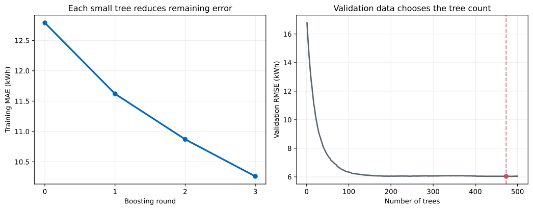
Read the panels separately. The left panel explains the mechanism: each new tree reduces error on the rows it studies. The right panel explains model selection: improvement on separate data eventually stops. More training trees are not automatically better.

Refit and evaluate once on the test set

The validation set has now finished its job. Refit a new model with exactly 473 trees, using both training and validation rows. This gives the final model more data without changing the selected tree count.

combined = pd.concat([train, validation], ignore_index=True)

final_model = GradientBoostingRegressor(
    n_estimators=best_stage,
    learning_rate=0.05,
    max_depth=3,
    min_samples_leaf=4,
    random_state=84,
)
final_model.fit(combined[features], combined["demand_kwh"])

Now use the untouched test set once. Compare the model with a basic baseline that always predicts the combined training mean:

from sklearn.metrics import mean_absolute_error

X_test = test[features]
y_test = test["demand_kwh"]
test_prediction = final_model.predict(X_test)

baseline_prediction = np.full(len(y_test), combined["demand_kwh"].mean())
print(f"mean-only baseline MAE: {mean_absolute_error(y_test, baseline_prediction):.2f} kWh")
print(f"gradient boosting MAE:  {mean_absolute_error(y_test, test_prediction):.2f} kWh")
print(f"gradient boosting RMSE: {root_mean_squared_error(y_test, test_prediction):.2f} kWh")

mean-only baseline MAE: 13.82 kWh
gradient boosting MAE:  4.03 kWh
gradient boosting RMSE: 5.24 kWh

The fitted model’s typical absolute miss is 4.03 kWh on this synthetic test set, compared with 13.82 kWh for the mean-only baseline. RMSE is higher than MAE because several larger errors receive more weight. These values describe this generated dataset only; they do not guarantee performance on a real building.

Inspect individual predictions as well as aggregate metrics:

preview = pd.DataFrame({
    "actual_kwh": y_test.iloc[:5].to_numpy(),
    "predicted_kwh": test_prediction[:5].round(1),
})
preview

   actual_kwh  predicted_kwh
0      112.21          113.4
1      128.88          132.3
2      141.32          139.0
3      137.66          137.3
4      135.30          133.5

The fourth displayed prediction is close: 137.3 versus 137.66 kWh. The second misses by about 3.4 kWh. A preview cannot replace a metric, but it helps confirm that columns have the expected units and that predictions are plausible numbers.

Common mistakes and troubleshooting

Fitting each tree to the original target. That creates several similar trees rather than a boosting sequence. After the baseline, every new tree must fit the current residuals or the appropriate loss gradient.

Adding the full correction when a learning rate is configured. The update must multiply the tree prediction by learning_rate. Leaving out that multiplication makes the manual loop disagree with the estimator and can take steps that are too large.

Selecting the tree count on test data. Use validation data or a documented cross-validation plan for model choices. Keep test data for the final evaluation.

Expecting training error to reveal overfitting. Training error often keeps falling as trees are added. Monitor validation error with staged_predict. The estimator’s official API documentation lists this generator specifically for predictions at each stage.

Using deep trees without a reason. Deep correction trees can learn narrow patterns and noise. Start with shallow trees and a small learning rate. Change one group of settings at a time, then compare on the same validation plan.

Ignoring time order in a forecasting project. Random splitting is convenient for this controlled synthetic example. For future-demand prediction, train on earlier timestamps and validate on later timestamps so the evaluation matches how the model will be used.

Getting different results on a rerun. Check the dataset, package versions, and all random_state values. This tutorial fixes the synthetic-data seed and estimator seeds. Small version changes can still change fitted tree details.

Recap

Gradient boosting is easier to understand as repeated correction than as one large model. Start with a simple prediction, measure what remains wrong, fit a small tree to those residuals, and add a scaled correction.

The learning rate controls the size of each correction. Tree depth controls how complex one correction can be. The number of trees controls how many correction rounds the ensemble receives. These settings work together, so choose them with data that was not used to fit the trees.

In this lesson, three visible stump corrections reduced training MAE from 12.79 to 10.26 kWh. A full validation curve selected 473 trees. After refitting, the final model achieved 4.03 kWh MAE on an untouched synthetic test set. The durable workflow is not that exact number. It is the separation of roles: train to learn, validate to choose, and test once to estimate final performance.