How to Add Attention to a GRU in PyTorch for Classification

A cold-room monitor records temperature, door state, and vibration at each time step. Most readings are routine, but one short combination of high temperature, an open door, and strong vibration may determine whether the whole sequence needs review. A classifier should keep the useful moment instead of treating every time step as equally important.

To add attention to a GRU in PyTorch, return the GRU hidden state for every valid step, score each state with a small neural network, mask padded positions before softmax, and take the weighted sum of states. Feed that context vector to a classifier and return the weights so you can test that padding receives zero weight.

This tutorial builds that path from input shapes to a trained binary classifier. If recurrent input shapes are new to you, read how to shape time-series data for an LSTM first. A GRU and an LSTM use different internal gates, but both expect the same basic sequence shape.

Setup and Prerequisites

You need Python 3.11 or newer and basic experience with Python functions and NumPy-style arrays. You do not need to know the equations inside a gated recurrent unit (GRU). For this lesson, a GRU is a layer that reads a sequence in order and produces a learned hidden state, or numeric summary, at each step.

Create a virtual environment and install the packages:

python -m venv .venv
source .venv/bin/activate
python -m pip install torch numpy pandas matplotlib

On Windows PowerShell, activate the environment with .venv\Scripts\Activate.ps1. If your system needs a platform-specific PyTorch package, use the command from the official PyTorch installation guide. The executed tutorial used Python 3.13.2, PyTorch 2.12.0, NumPy 2.5.1, pandas 3.0.3, and Matplotlib 3.11.0.

Download cold_room_sequences.csv and save it beside your Python file. This original synthetic dataset contains 1,200 fictional sensor sequences and is released under CC0-1.0. A fixed random seed created every value, so the data can be rebuilt exactly. It contains no readings from a real building or device.

The teaching rule is intentionally clear. A positive sequence contains one time step where temperature, door state, and vibration are all high. Negative sequences include realistic decoys, such as high temperature with a closed door or an open door with normal temperature. This makes the data useful for checking the attention mechanism, but not for estimating performance on real equipment.

Mental Model: Read, Weigh, and Combine

The model performs three jobs in order:

1. The GRU reads the sequence and creates one hidden state per time step.
2. The attention layer gives each valid hidden state a score and converts all scores to weights that sum to 1.
3. A weighted sum combines the hidden states into one context vector, which the final layer uses for classification.

Suppose a sequence has 12 steps and each GRU state has 20 numbers. The GRU output has shape (batch, 12, 20). Attention returns one weight per step with shape (batch, 12). The weighted sum removes the time dimension, leaving a context with shape (batch, 20).

This is attention pooling: it reduces a variable-length sequence to one fixed-width vector. It is different from self-attention, where every position builds a new representation by reading other positions. To study that second calculation, see scaled dot-product attention in NumPy.

Sequences have different lengths, so a batch also contains padding. Padding is a placeholder added after a shorter sequence. It is not a sensor reading. The attention layer must assign it zero weight, or the context vector will include invented steps.

Inspect and Prepare the Sequence Data

Start by loading the CSV and checking its size. The event_step column records where the synthetic generator inserted the positive pattern. It is included only for auditing and the final chart; never give it to the model because it reveals the answer.

import numpy as np
import pandas as pd
import torch

data = pd.read_csv("cold_room_sequences.csv")
feature_columns = ["temperature_c", "door_open", "vibration_g"]

print("rows:", len(data))
print("sequences:", data["sequence_id"].nunique())
print(data.groupby("sequence_id").size().agg(["min", "max"]))
print(data.head(4).to_string(index=False))

rows: 15427
sequences: 1200
min     8
max    18
sequence_id split  step  temperature_c  door_open  vibration_g  risk_label  event_step
  room_0000 train     0          3.589          0        0.204           0          -1
  room_0000 train     1          3.721          0        0.214           0          -1
  room_0000 train     2          3.677          0        0.192           0          -1
  room_0000 train     3          3.384          0        0.216           0          -1

Each CSV row is one time step. The 1,200 sequences range from 8 to 18 steps, so 18 becomes the padded width. The supplied split keeps 960 sequences for training and 240 for testing. Splitting by sequence_id, rather than by row, prevents time steps from the same sequence appearing in both sets.

Feature scales are different: temperature is near 4, door state is 0 or 1, and vibration is near 0.2. Calculate the mean and standard deviation from training rows only. Using test statistics would let information from the held-out set influence preprocessing.

train_rows = data[data["split"] == "train"]
means = train_rows[feature_columns].mean().to_numpy(np.float32)
scales = train_rows[feature_columns].std(ddof=0).to_numpy(np.float32)
max_length = int(data.groupby("sequence_id").size().max())

The helper below changes a list of sequence IDs into four tensors. inputs holds scaled features, lengths stores each real length, valid_steps is True for real data and False for padding, and labels holds one target per sequence.

def tensorize(frame, sequence_ids, means, scales, max_length):
    inputs = np.zeros((len(sequence_ids), max_length, 3), dtype=np.float32)
    lengths = np.zeros(len(sequence_ids), dtype=np.int64)
    labels = np.zeros(len(sequence_ids), dtype=np.float32)
    grouped = frame.groupby("sequence_id", sort=False)

    for row, sequence_id in enumerate(sequence_ids):
        sequence = grouped.get_group(sequence_id)
        values = sequence[feature_columns].to_numpy(np.float32)
        length = len(values)
        inputs[row, :length] = (values - means) / scales
        lengths[row] = length
        labels[row] = sequence["risk_label"].iloc[0]

    steps = np.arange(max_length)[None, :]
    valid_steps = steps < lengths[:, None]
    return (
        torch.from_numpy(inputs),
        torch.from_numpy(lengths),
        torch.from_numpy(valid_steps),
        torch.from_numpy(labels),
    )

Build the two sets from the predefined split. Keep the IDs in the same order as their tensors so that you can connect a prediction back to its source rows.

train_ids = data.loc[data["split"] == "train", "sequence_id"].drop_duplicates().tolist()
test_ids = data.loc[data["split"] == "test", "sequence_id"].drop_duplicates().tolist()

train = tensorize(data, train_ids, means, scales, max_length)
test = tensorize(data, test_ids, means, scales, max_length)

print("test inputs:", tuple(test[0].shape))
print("test lengths:", tuple(test[1].shape))

test inputs: (240, 18, 3)
test lengths: (240,)

There are 240 test sequences, each stored in an 18-step container with three features. The separate length tensor tells the model where each real sequence ends.

Build a Padding-Aware Attention Layer

Create the attention module before the full classifier. The first linear layer learns a transformation of each GRU state. tanh adds a nonlinear step, and the second linear layer reduces each transformed state to one score.

from torch import nn

class MaskedAttentionPool(nn.Module):
    def __init__(self, hidden_size):
        super().__init__()
        self.projection = nn.Linear(hidden_size, hidden_size)
        self.scorer = nn.Linear(hidden_size, 1, bias=False)

    def forward(self, states, valid_steps):
        scores = self.scorer(torch.tanh(self.projection(states))).squeeze(-1)
        scores = scores.masked_fill(
            ~valid_steps,
            torch.finfo(scores.dtype).min,
        )
        weights = torch.softmax(scores, dim=1)
        context = torch.bmm(weights.unsqueeze(1), states).squeeze(1)
        return context, weights

The Boolean mask uses True for real steps. The ~ operator reverses it, so masked_fill replaces padding scores with the smallest available value for the score’s floating-point type. Softmax turns those extremely negative scores into zero weights and normalizes the valid weights to a total of 1.

torch.bmm performs a batch of matrix multiplications. After unsqueeze(1), weights have shape (batch, 1, time). Multiplying by states with shape (batch, time, hidden) produces (batch, 1, hidden). The final squeeze removes the size-one dimension.

Returning weights is important. The classifier needs only context, but the weights let you test the mask and inspect which states affected one decision. They are a diagnostic for this pooling operation, not proof of every reason behind a model prediction.

Connect Attention to the GRU

Now place the attention module after the GRU. The model uses batch_first=True, so inputs and outputs follow (batch, time, feature). This layout is documented by PyTorch’s current nn.GRU reference.

from torch.nn.utils.rnn import pack_padded_sequence, pad_packed_sequence

class GRUAttentionClassifier(nn.Module):
    def __init__(self, feature_count=3, hidden_size=20):
        super().__init__()
        self.gru = nn.GRU(feature_count, hidden_size, batch_first=True)
        self.attention = MaskedAttentionPool(hidden_size)
        self.classifier = nn.Linear(hidden_size, 1)

    def forward(self, inputs, lengths, valid_steps):
        packed = pack_padded_sequence(
            inputs,
            lengths.cpu(),
            batch_first=True,
            enforce_sorted=False,
        )
        packed_states, _ = self.gru(packed)
        states, _ = pad_packed_sequence(
            packed_states,
            batch_first=True,
            total_length=inputs.shape[1],
        )
        context, weights = self.attention(states, valid_steps)
        logits = self.classifier(context).squeeze(-1)
        return logits, weights

Packing tells the GRU to skip padded steps instead of processing zeros as if they were readings. PyTorch’s pack_padded_sequence accepts unsorted lengths when enforce_sorted=False; lengths must be on the CPU when supplied as a tensor. Unpacking restores the rectangular (batch, 18, hidden) shape needed by the attention layer.

The classifier returns logits, which are unrestricted scores before a sigmoid conversion. BCEWithLogitsLoss combines sigmoid and binary cross-entropy in one numerically stable function during training.

Train and Test the Classifier

Set every random seed before creating the model. The reproducible build also selects deterministic PyTorch operations and uses one CPU thread. Batches still change order between epochs, but the seeded generator makes that order repeatable in the tested environment.

import random

random.seed(20260715)
np.random.seed(20260715)
torch.manual_seed(20260715)
torch.set_num_threads(1)
torch.use_deterministic_algorithms(True)

model = GRUAttentionClassifier()
optimizer = torch.optim.Adam(model.parameters(), lr=0.008)
loss_function = nn.BCEWithLogitsLoss()
generator = torch.Generator().manual_seed(20260715)

def batches(size, batch_size):
    order = torch.randperm(size, generator=generator)
    for start in range(0, size, batch_size):
        yield order[start:start + batch_size]

model.train()
for epoch in range(1, 25):
    total_loss = 0.0
    correct = 0

    for index in batches(len(train_ids), 64):
        optimizer.zero_grad()
        logits, _ = model(train[0][index], train[1][index], train[2][index])
        loss = loss_function(logits, train[3][index])
        loss.backward()
        optimizer.step()

        total_loss += float(loss.detach()) * len(index)
        correct += int(((logits >= 0).float() == train[3][index]).sum())

    if epoch == 24:
        print(
            f"epoch {epoch}: loss={total_loss / len(train_ids):.4f}, "
            f"accuracy={correct / len(train_ids):.4f}"
        )

The core update has five steps: clear old gradients, run the model, calculate loss, backpropagate, and update the parameters. The two totals accumulate the loss and number of correct predictions across each epoch. The final training line was:

epoch 24: loss=0.0002, accuracy=1.0000

This is training performance, so it cannot tell us how the model handles held-out sequences. Evaluate the test tensors without recording gradients, then calculate loss, accuracy, and the four entries of the confusion matrix:

model.eval()
with torch.no_grad():
    test_logits, test_weights = model(test[0], test[1], test[2])
    test_loss = loss_function(test_logits, test[3])
    probabilities = torch.sigmoid(test_logits)
    predictions = (probabilities >= 0.5).float()

confusion = {
    "true_negative": int(((test[3] == 0) & (predictions == 0)).sum()),
    "false_positive": int(((test[3] == 0) & (predictions == 1)).sum()),
    "false_negative": int(((test[3] == 1) & (predictions == 0)).sum()),
    "true_positive": int(((test[3] == 1) & (predictions == 1)).sum()),
}

print(f"parameters: {sum(parameter.numel() for parameter in model.parameters()):,}")
print(f"test: loss={float(test_loss):.4f}, accuracy={(predictions == test[3]).float().mean():.4f}")
print("confusion:", confusion)

parameters: 1,961
test: loss=0.0002, accuracy=1.0000
confusion: {'true_negative': 120, 'false_positive': 0, 'false_negative': 0, 'true_positive': 120}

All 240 held-out synthetic sequences were classified correctly: 120 negatives and 120 positives. That perfect result means the model learned this deliberately simple generated rule. It does not show that the same architecture will classify noisy real sensor data perfectly. A real project needs representative measurements, labels created through a valid process, and evaluation across devices and operating conditions.

Next, test the attention properties directly. The earlier torch.no_grad() block already produced test_weights, so these checks do not need another model call.

padded_weights = test_weights.masked_select(~test[2])
row_sums = test_weights.sum(dim=1)

print("largest padding weight:", float(padded_weights.abs().max()))
print("largest row-sum error:", float((row_sums - 1).abs().max()))

largest padding weight: 0.0
largest row-sum error: 1.1920928955078125e-07

Padding received exactly zero weight. Every row total was within about 0.00000012 of 1; this tiny difference is normal floating-point rounding. These checks test the layer’s numeric rules separately from classification accuracy.

Read One Sequence’s Attention Weights

The chart below uses a correctly classified eight-step test sequence. Step 6 contains the generated combination: 9.695°C, an open door, and vibration of 0.881 g. The model predicted the risk class with probability 0.9998.

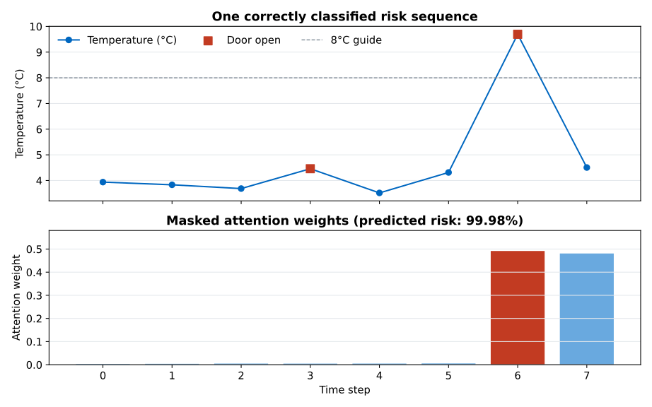
The largest attention weight, 0.4918, occurs at the inserted event. Step 7 receives the nearly equal weight 0.4809. Because this is a one-directional GRU, its state at step 7 can still carry information from step 6. This is an important limit on interpretation: attention scores GRU states, and each state already summarizes the sequence up to that point. A large weight at a later step does not mean the raw step alone caused the prediction.

The remaining six steps share less than 3% of the total weight. For this example, attention pooling concentrates the context on the event state and the next state that remembers it. The mask test is still separate: if this sequence had padding after step 7, those placeholder positions would receive exactly zero.

Common Mistakes and Troubleshooting

Masking after softmax. If you set padding weights to zero after normalization, the remaining weights no longer sum to 1. Mask the scores first, then call softmax.

Reversing the mask. This lesson uses True for valid steps. masked_fill changes positions where its mask is True, which is why the code passes ~valid_steps. Print one mask row beside its length when debugging.

Packing without CPU lengths. pack_padded_sequence requires a length tensor on the CPU. Use lengths.cpu() even when inputs and model parameters are on an accelerator.

Sorting data unnecessarily. The default packing behavior expects decreasing lengths. Setting enforce_sorted=False lets PyTorch handle an ordinary shuffled batch. Sort only when an export or downstream workflow requires it.

Sending label information into the model. Do not include risk_label, event_step, split, or sequence_id in feature_columns. They describe the target, audit data, or bookkeeping rather than sensor inputs.

Splitting CSV rows instead of sequences. Random row splitting leaks readings from one sequence across training and test data. Split unique sequence IDs first, then collect all rows belonging to each ID.

Assuming attention is a complete explanation. The weights show how this layer mixed GRU states. Those states already contain earlier information, and other model parameters also affect the prediction. Treat weights as a useful inspection signal, not a causal explanation.

Seeing nan weights. A fully masked row has no valid value for softmax. Verify that every length is at least 1 and that each mask contains at least one True value.

Recap

Adding attention to a GRU sequence classifier requires a clear shape and masking path:

1. Store a batch as (batch, time, feature) plus one real length per sequence.
2. Pack the padded inputs so the GRU skips placeholder steps.
3. Unpack all GRU states to a common time width.
4. Learn one score per state and mask padding before softmax.
5. Take the weighted sum to create one context vector per sequence.
6. Classify the context and return the weights for numeric tests and careful inspection.

The durable mental model is read, weigh, and combine. The GRU reads in order, attention weighs valid hidden states, and the context combines them into the fixed-size input needed by a classifier. Keep packing and masking as separate safeguards: packing protects the recurrent calculation, while masking protects the attention calculation.