A fault detector can be 93% accurate and still miss every fault. That happens when about 93% of the rows are normal: a model that always answers “normal” receives a high accuracy score while providing no useful warning.

To handle imbalanced classes with XGBoost, make stratified train, validation, and test splits; calculate scale_pos_weight from the training labels; and compare the weighted model with an unweighted baseline using precision, recall, and average precision. Choose the decision threshold on validation data for the required recall, then measure the locked workflow once on the untouched test set.

This tutorial applies that process to fictional pump-health checks. The task is binary classification: each row belongs to one of two classes, fault within seven days (1) or no fault (0). You will see why class weighting and threshold tuning solve different parts of the problem—and why neither removes the need to count false alerts.

Setup and inspect the rare class

You should be able to run a Python script or notebook cell and recognize rows and columns in a table. You do not need to know boosting mathematics. If training features, targets, and test sets are new terms, start with your first machine learning model.

Create a virtual environment so this lesson’s packages remain separate from other Python projects. On macOS or Linux, run:

python -m venv .venv
source .venv/bin/activate
python -m pip install numpy pandas scikit-learn xgboost matplotlib

On Windows PowerShell, activate with .venv\Scripts\Activate.ps1 instead. The executed build used Python 3.13.2, NumPy 2.5.1, pandas 3.0.3, scikit-learn 1.9.0, XGBoost 3.3.0, and Matplotlib 3.11.0.

The lesson uses pump_fault_checks.csv. It is an original synthetic dataset released under CC0-1.0. All 5,000 check identifiers, readings, service intervals, and outcomes are fictional. A fixed NumPy seed makes the build reproducible; the results do not describe a real maintenance system.

Load the file and keep the first view small. These columns show the check ID, two sensor readings, the service interval, and the target:

import pandas as pd

pumps = pd.read_csv(
    "https://datatweets.com/datasets/blog/"
    "handle-imbalanced-classes-xgboost-python/pump_fault_checks.csv"
)

columns_to_view = [
    "check_id",
    "motor_temperature_c",
    "vibration_mm_s",
    "days_since_service",
    "fault_within_7_days",
]
print(pumps[columns_to_view].head().to_string(index=False))

   check_id  motor_temperature_c  vibration_mm_s  days_since_service  fault_within_7_days
PUMP-00001                 47.9            1.69                44.7                      0
PUMP-00002                 59.5            2.97                58.9                      0
PUMP-00003                 55.4            4.34               107.4                      0
PUMP-00004                 58.2            8.23               109.5                      0
PUMP-00005                 57.8            2.70                95.5                      0

The features are the values available to the model when it makes a prediction. The target is the answer it learns to predict. Here, fault_within_7_days=1 is the positive class because it is the event that should trigger attention.

Now count both target values before fitting anything:

target = "fault_within_7_days"

print(pumps[target].value_counts().sort_index())
print(f"fault rate: {pumps[target].mean():.3%}")

fault_within_7_days
0    4657
1     343
Name: count, dtype: int64
fault rate: 6.860%

The data is imbalanced because one class is much less common than the other. There are about 13.6 normal checks for each fault check. Imbalance is not automatically an error; many real events are rare. The problem is using an evaluation or training choice that allows the common class to hide the rare one.

Understanding ranking, class weight, and thresholds

Ranking, class weighting, and thresholding are related, but each has a different job.

First, predict_proba() returns a numeric score between 0 and 1 for each class. A useful model gives higher positive-class scores to faults than to normal checks. A precision-recall curve evaluates that ranking across many possible decision thresholds.

Second, scale_pos_weight changes how much positive training rows contribute to XGBoost’s objective, the quantity that training tries to reduce. With a value above 1, errors on positive rows receive more weight. The current XGBoost parameter reference suggests the number of negative training instances divided by the number of positive training instances as a typical value to consider for imbalanced classes. It is a starting point, not a guaranteed best setting.

Third, a decision threshold turns scores into actions. With threshold 0.50, a score at or above 0.50 becomes a fault alert. Lowering the threshold sends more pumps for inspection. It usually finds more real faults and also creates more false alerts.

The two main alert metrics make that tradeoff visible:

precision = true faults found / all fault alerts
recall    = true faults found / all actual faults

High precision means the inspection queue contains fewer false alerts. High recall means fewer real faults were missed. Accuracy mixes the common and rare classes into one fraction, so it can look strong while recall is zero.

Give each data split one job

The threshold is a model choice, so it must not be selected on the final test data. We will use 3,000 training rows to fit the trees, 1,000 validation rows to choose the threshold, and 1,000 test rows to measure the completed process once.

The following code names the six numeric features, then uses stratify in both splits. Stratification keeps a similar positive-class rate in every part:

from sklearn.model_selection import train_test_split

features = [
    "pump_age_months",
    "operating_load_pct",
    "motor_temperature_c",
    "vibration_mm_s",
    "starts_24h",
    "days_since_service",
]

development, test = train_test_split(
    pumps,
    test_size=1000,
    random_state=20_260_722,
    stratify=pumps[target],
)
train, validation = train_test_split(
    development,
    test_size=1000,
    random_state=20_260_722,
    stratify=development[target],
)

print(len(train), len(validation), len(test))

3000 1000 1000

This random split suits independent fictional checks generated from one stable process. For repeated readings from real pumps, a group split may be safer so one pump does not appear in both training and test data. For future-fault prediction, a time-based split may also be necessary. Match the split to how new data will arrive.

Define a controlled model comparison

The complete dataset contains 4,657 normal checks out of 5,000 rows. A deliberately useless rule that always predicts 0 would therefore be 93.1% accurate while finding none of the faults. We will include that rule in the final test comparison, after every model choice is fixed.

Define one model factory next. Keeping all other settings fixed lets us compare unweighted and weighted training without accidentally changing tree depth or the number of trees:

from xgboost import XGBClassifier

def new_classifier(scale_pos_weight=1.0):
    return XGBClassifier(
        objective="binary:logistic",
        eval_metric="logloss",
        tree_method="hist",
        n_estimators=240,
        learning_rate=0.045,
        max_depth=4,
        min_child_weight=5,
        subsample=0.9,
        colsample_bytree=0.9,
        reg_lambda=2.0,
        scale_pos_weight=scale_pos_weight,
        random_state=20_260_722,
        n_jobs=1,
    )

objective="binary:logistic" produces scores for binary classification, while hist selects XGBoost’s histogram tree method. The remaining settings are fixed teaching choices for this dataset, not universal defaults. Because class weighting can affect probability calibration, treat the values returned by predict_proba() as ranking scores unless a separate calibration check supports a probability interpretation.

Add class weight from training labels only

Calculate the suggested ratio from train, not from the complete dataset. Test-label counts belong to the final evaluation and should not influence training choices:

negative_count = (train[target] == 0).sum()
positive_count = (train[target] == 1).sum()
class_ratio = negative_count / positive_count

print(negative_count, positive_count)
print(f"scale_pos_weight: {class_ratio:.3f}")

2794 206
scale_pos_weight: 13.563

There are 2,794 negative and 206 positive training rows. The ratio tells XGBoost to give each positive row about 13.6 times the weight of a negative row in the training objective.

Fit one unweighted classifier and one otherwise identical classifier with that ratio. Do not inspect the test results yet:

unweighted_model = new_classifier()
weighted_model = new_classifier(scale_pos_weight=class_ratio)

unweighted_model.fit(train[features], train[target])
weighted_model.fit(train[features], train[target])

The two fitted models differ only in scale_pos_weight. That controlled comparison will show what weighting changed without confusing its effect with a different depth, learning rate, or train/test split.

Choose an operating threshold on validation data

Suppose the maintenance plan asks the model to find at least 80% of known faults in validation data. We will choose the highest-precision threshold that meets that recall target. The scikit-learn precision_recall_curve documentation defines each returned threshold as the score at or above which a row is positive.

Generate validation scores first. The final test labels remain untouched:

import numpy as np
from sklearn.metrics import precision_recall_curve

validation_score = weighted_model.predict_proba(
    validation[features]
)[:, 1]
precision, recall, thresholds = precision_recall_curve(
    validation[target], validation_score
)

eligible = np.flatnonzero(recall[:-1] >= 0.80)
best_precision = precision[eligible].max()
best_candidates = eligible[np.isclose(precision[eligible], best_precision)]
best_index = best_candidates[np.argmax(thresholds[best_candidates])]

chosen_threshold = thresholds[best_index]
print(f"threshold:            {chosen_threshold:.3f}")
print(f"validation precision: {precision[best_index]:.3f}")
print(f"validation recall:    {recall[best_index]:.3f}")

threshold:            0.222
validation precision: 0.152
validation recall:    0.809

The selected threshold is about 0.222, far below 0.50. This does not mean that every score above 0.222 represents a 22.2% real-world fault probability. Weighting changes the training objective, and these scores have not been calibrated. Here, the number is an operating cutoff chosen from validation evidence.

Measure the locked workflow on test data

We have now fixed the models, class weight, and threshold. Generate test scores once and compare the all-normal rule with three model decisions:

from sklearn.metrics import (
    accuracy_score,
    confusion_matrix,
    precision_score,
    recall_score,
)

unweighted_score = unweighted_model.predict_proba(test[features])[:, 1]
weighted_test_score = weighted_model.predict_proba(test[features])[:, 1]

def summarize(name, score, threshold_value):
    prediction = (score >= threshold_value).astype(int)
    tn, fp, fn, tp = confusion_matrix(
        test[target], prediction, labels=[0, 1]
    ).ravel()
    return {
        "method": name,
        "accuracy": accuracy_score(test[target], prediction),
        "precision": precision_score(
            test[target], prediction, zero_division=0
        ),
        "recall": recall_score(test[target], prediction),
        "FP": fp,
        "FN": fn,
        "TP": tp,
    }

comparison = pd.DataFrame([
    summarize("all normal", np.zeros(len(test)), 0.50),
    summarize("unweighted, 0.50", unweighted_score, 0.50),
    summarize("weighted, 0.50", weighted_test_score, 0.50),
    summarize(
        f"weighted, {chosen_threshold:.3f}",
        weighted_test_score,
        chosen_threshold,
    ),
])
print(comparison.round(3).to_string(index=False))

             method  accuracy  precision  recall  FP  FN  TP
         all normal     0.931      0.000   0.000   0  69   0
   unweighted, 0.50     0.929      0.438   0.101   9  62   7
     weighted, 0.50     0.845      0.231   0.536 123  32  37
    weighted, 0.222     0.702      0.160   0.783 283  15  54

The all-normal rule is correct on 931 normal checks and wrong on all 69 faults. Its 93.1% accuracy is not useful evidence for a fault detector.

At the default threshold, the unweighted model creates 16 alerts, 7 of which are real faults. Weighting raises recall from 10.1% to 53.6%, but precision falls from 43.8% to 23.1%. It finds 30 additional faults and adds 114 false alerts. Whether that exchange is acceptable depends on inspection cost and capacity, not on a universal rule.

The validation-selected threshold finds 54 of the 69 test faults, for 78.3% test recall, and misses 15. Recall is slightly below the 80% validation target because validation and test contain different samples.

The cost is visible: 283 normal checks also enter the 337-row inspection queue. Precision is 16.0%, so roughly one in six alerts is a fault in this synthetic test. This may be useful when missed faults are expensive and inspections are cheap. It may be unusable when only a small number of inspections can be completed.

Accuracy falls to 70.2% even though the workflow now finds far more faults. This is why accuracy alone points in the wrong direction for this operating goal.

Average precision (AP) summarizes the precision-recall ranking across thresholds. Higher is better. Unlike a threshold-specific metric, it evaluates whether positives generally receive higher scores than negatives. The official scikit-learn documentation defines AP as a recall-weighted mean of precision values.

from sklearn.metrics import average_precision_score

print(
    "unweighted AP:",
    round(average_precision_score(test[target], unweighted_score), 3),
)
print(
    "weighted AP:  ",
    round(average_precision_score(test[target], weighted_test_score), 3),
)

unweighted AP: 0.271
weighted AP:   0.239

Class weighting did not improve test AP in this run. It made the 0.50 operating point much more sensitive to faults, but the unweighted model ranked test rows slightly better overall. That result is important: scale_pos_weight is a candidate to evaluate, not a switch that guarantees a better model.

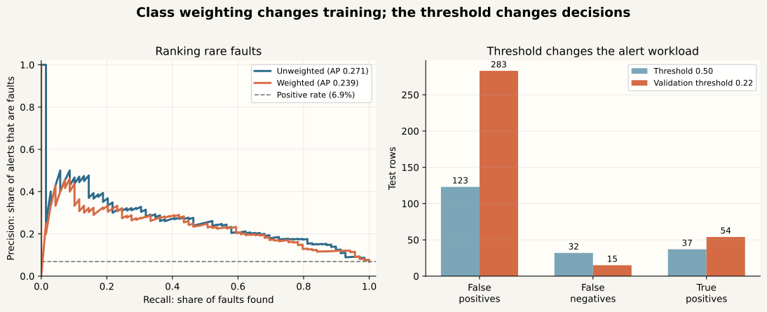
Read the left panel as a ranking comparison across thresholds. Both curves sit above the dashed 6.9% positive-rate reference for much of the range, but the unweighted curve has the higher AP. Read the right panel as a workload comparison: lowering the threshold catches more faults by asking for many more inspections.

The final step turns scores into an inspectable queue. Sort by the weighted score so the highest-priority checks appear first, while keeping the chosen threshold as an explicit boolean column:

inspection_queue = pd.DataFrame({
    "check_id": test["check_id"].to_numpy(),
    "fault_score": weighted_test_score,
    "send_for_inspection": weighted_test_score >= chosen_threshold,
    "actual_fault": test[target].to_numpy(),
}).sort_values("fault_score", ascending=False)

print(inspection_queue.head().round(3).to_string(index=False))

   check_id  fault_score  send_for_inspection  actual_fault
PUMP-01439        0.962                 True             0
PUMP-03062        0.954                 True             0
PUMP-00526        0.940                 True             0
PUMP-04781        0.938                 True             1
PUMP-01795        0.938                 True             0

actual_fault is included only because this is an evaluated historical test set. A live queue would not know the future outcome at prediction time. Keep it out of the input features and add it later only when outcomes arrive for monitoring.

Common mistakes and practical fixes

Using accuracy as the main success measure. The all-normal rule reached 93.1% accuracy with zero recall. Start with the confusion-matrix counts, precision, recall, and a precision-recall curve. Select metrics from the real cost of false positives and false negatives.

Calculating class weight before the split. Use training labels only. The ratio may look similar on the complete data, but a clean boundary makes the workflow easier to audit and avoids using final evaluation information in model setup.

Treating negative / positive as the only valid weight. XGBoost documents it as a typical value to consider. Compare it with 1.0 and, if needed, other values on validation data. A smaller weight may provide a better inspection workload; a larger one may raise recall further and reduce precision.

Changing the threshold on test data. If you repeatedly inspect test recall and adjust the cutoff, the test set becomes part of model development. Choose the threshold on validation data or within cross-validation, then evaluate it once on the test set.

Assuming weighted scores are calibrated probabilities. Class weighting changes the loss. A score can rank cases usefully without matching observed event frequencies. If the number must communicate risk, evaluate probability calibration separately; probability calibration with scikit-learn shows that workflow.

Oversampling before the split. Copying rare rows first can place duplicates in both training and test data. Split the original rows first, then apply any resampling only inside the training process. Group or time boundaries still need protection.

Ignoring the alert count. A metric target can create more alerts than a team can inspect. Report false positives and predicted-positive counts next to recall. A threshold is an operational decision, not only a model parameter.

Getting different results. Confirm the published CSV, package versions, split seed, feature order, and model settings. Keep n_jobs=1 for the closest reproduction. Small floating-point differences can still occur on another platform.

Recap: what to carry into the next rare-event model

An imbalanced target needs a workflow, not one special parameter. Start by counting the classes and showing what an all-common-class rule would score. Preserve separate training, validation, and test roles. Then compare class weighting on the same rows and model settings.

Use average precision and the precision-recall curve to judge ranking across thresholds. Use precision, recall, and confusion-matrix counts to judge one operating threshold. Finally, translate the chosen threshold into a workload that people or systems can actually handle.

In this synthetic pump example, the unweighted model had higher average precision, while class weighting increased recall at the default threshold. A validation-selected threshold found 54 of 69 test faults but also created 283 false alerts. The durable conclusion is not that 13.563 or 0.222 is correct elsewhere. It is that weighting changes how XGBoost learns, the threshold changes which rows trigger action, and untouched test data shows the cost of both choices.