TensorFlow and Keras: A Practical Introduction to Neural Networks

Every model on this site so far has answered a question scikit-learn was built for: given a table of features that already mean something — a wine’s acidity, a patient’s BMI, a tumor’s radius — predict a label or a number. But some data doesn’t arrive as a tidy table of meaningful columns. A photograph is a grid of raw pixel brightnesses. Audio is a wall of amplitude samples. Nothing about pixel number 407 has an obvious meaning on its own, the way “average glucose” does. You need a model that can learn its own useful features from raw numbers, not just combine features you’ve already engineered — and that’s the job neural networks do.

If you’ve used scikit-learn’s fit/predict pattern, this is going to feel familiar on the surface: our scikit-learn overview post covers a .fit() call, then a .predict() call, for every estimator it ships. TensorFlow’s Keras API keeps that same two-verb shape. What’s different is what happens inside .fit() this time — instead of solving one equation or storing the training data, Keras is nudging thousands of numbers, a little at a time, over and over, across many passes through the data. That’s a genuinely different mental model, and it’s easy to run the code without ever forming it. This post builds that model first, then trains a real, small neural network end to end: load real image data, normalize it, stack a couple of layers, compile the model, train it, and grade it honestly on data it never saw.

The Mental Model: A Stack of Transformations, Nudged Until They’re Right

A neural network is not one formula — it’s several small ones, chained together, each one learned:

1. Data goes in as plain numbers. An image is just a grid of brightness values; there’s no separate “feature engineering” step required before the network can use it.
2. Each layer takes numbers in and hands different numbers out. A layer multiplies its input by a matrix of weights, adds a bias, and passes the result through a small nonlinear function called an activation. That’s the entire operation, repeated layer after layer.
3. The stack’s last layer turns those numbers into a guess — a probability for each possible answer, in a classification problem like this one.
4. Training compares the guess to the real answer with a loss function, a single number that’s small when the guess was close and large when it was badly wrong.
5. Every weight in every layer gets nudged a little, in the direction that would have made the loss smaller. This nudging step, computed layer by layer working backward from the loss, is called backpropagation — you won’t need its calculus to use it, only the fact that it’s how the nudging direction gets computed.
6. Repeat steps 3–5 many times over the whole training set. One full pass through all the training data is called an epoch. A network usually needs several epochs before its guesses are any good.

Compare that to scikit-learn’s LinearRegression, which solves for its weights in one shot, or KNeighborsClassifier, which does no learning at all and just stores the data. A neural network’s .fit() call is doing real, iterative work on every one of those epochs — which is exactly why, later in this post, you’ll watch the loss and accuracy change epoch by epoch instead of appearing all at once.

A Dataset You Can Reproduce

This post uses MNIST, a dataset of 70,000 grayscale images of handwritten digits (0 through 9), each a tiny 28x28-pixel square. MNIST ships with TensorFlow itself — no download step of your own, no license to check, nothing to vendor — which also makes it the standard first dataset almost everyone uses to learn this exact workflow. Imagine you’re prototyping a mailroom scanner that reads the handwritten digits on an envelope and sorts it by postal code; recognizing one digit at a time from a small square image is exactly the sub-problem this dataset represents.

import tensorflow as tf

(X_train, y_train), (X_test, y_test) = tf.keras.datasets.mnist.load_data()
print("X_train.shape:", X_train.shape, "X_train.dtype:", X_train.dtype)
print("y_train.shape:", y_train.shape, "y_train.dtype:", y_train.dtype)
print("X_test.shape:", X_test.shape)
print("first label:", y_train[0])

X_train.shape: (60000, 28, 28) X_train.dtype: uint8
y_train.shape: (60000,) y_train.dtype: uint8
X_test.shape: (10000, 28, 28)
first label: 5

60,000 training images and 10,000 held-out test images, each 28 by 28 pixels, plus one label per image telling you which digit it actually is. y_train[0] being 5 means the very first training image is a handwritten 5. The pixels themselves are plain integers:

print("pixel value sample (row 7 of image 0):", X_train[0, 7])
print("min pixel value:", X_train.min(), "max pixel value:", X_train.max())

pixel value sample (row 7 of image 0): [  0   0   0   0   0   0   0  49 238 253 253 253 253 253 253 253 253 251
  93  82  82  56  39   0   0   0   0   0]
min pixel value: 0 max pixel value: 255

Row 7 of the first image is mostly 0 (black background) with a run of values near 253 (close to white) where the stroke of the digit passes through — that bright band is a cross-section of the handwritten 5. Every pixel in every image is an integer from 0 to 255, the standard 8-bit grayscale range. (The output in this post comes from TensorFlow 2.21.0 with Keras 3.15.0.)

Normalizing Pixel Values Before Training

Neural networks train on gradients — small, repeated nudges to every weight — and those nudges behave far better when the input numbers are small and centered near zero than when they range up into the hundreds. Raw pixel values from 0 to 255 are exactly the kind of large, skewed input that makes training slower and less stable. The fix is a simple rescale to the 0–1 range:

X_train_norm = X_train.astype("float32") / 255.0
X_test_norm = X_test.astype("float32") / 255.0
print("min after normalize:", X_train_norm.min(), "max after normalize:", X_train_norm.max())
print("dtype after normalize:", X_train_norm.dtype)

min after normalize: 0.0 max after normalize: 1.0
dtype after normalize: float32

Every pixel is now a float between 0.0 and 1.0 instead of an integer between 0 and 255. This isn’t the same scaling story as StandardScaler in the scikit-learn posts on this site — there, the concern was one feature’s huge range silently dominating a distance calculation. Here, the concern is a training-stability one specific to neural networks: large, differently-scaled inputs push the very first layer’s gradients to wildly different sizes, which makes the optimizer’s step size wrong for some weights and right for others at the same time. The gotchas section below shows exactly how much that costs in practice, with a real side-by-side run.

Stacking Layers with Sequential

Keras’s Sequential model is the simplest way to describe the “stack of transformations” from the mental model: you hand it an ordered list of layers, and each one’s output feeds directly into the next one’s input.

model = tf.keras.Sequential([
    tf.keras.layers.Input(shape=(28, 28)),
    tf.keras.layers.Flatten(),
    tf.keras.layers.Dense(128, activation="relu"),
    tf.keras.layers.Dense(10, activation="softmax"),
])
model.summary()

Model: "sequential"
┏━━━━━━━━━━━━━━━━━━━━━━━━━━━━━━━━━┳━━━━━━━━━━━━━━━━━━━━━━━━┳━━━━━━━━━━━━━━━┓
┃ Layer (type)                    ┃ Output Shape           ┃       Param # ┃
┡━━━━━━━━━━━━━━━━━━━━━━━━━━━━━━━━━╇━━━━━━━━━━━━━━━━━━━━━━━━╇━━━━━━━━━━━━━━━┩
│ flatten (Flatten)               │ (None, 784)            │             0 │
├─────────────────────────────────┼────────────────────────┼───────────────┤
│ dense (Dense)                   │ (None, 128)            │       100,480 │
├─────────────────────────────────┼────────────────────────┼───────────────┤
│ dense_1 (Dense)                 │ (None, 10)             │         1,290 │
└─────────────────────────────────┴────────────────────────┴───────────────┘
 Total params: 101,770 (397.54 KB)
 Trainable params: 101,770 (397.54 KB)
 Non-trainable params: 0 (0.00 B)

Read the stack top to bottom, matching the mental model: Input(shape=(28, 28)) declares the shape of one image, without a batch dimension. Flatten() reshapes each 28x28 image into a single row of 784 numbers, since Dense layers expect a flat vector, not a grid. The first Dense(128, activation="relu") is a hidden layer — it has no direct meaning of its own, but it’s where the network builds intermediate representations useful for telling digits apart; relu is the nonlinearity from step 2 of the mental model, and without one, stacking Dense layers would collapse mathematically into a single linear layer no matter how many you added. The final Dense(10, activation="softmax") is the output layer: 10 numbers, one per digit, and softmax forces them to be non-negative and sum to 1 — a genuine probability distribution over the 10 possible digits. 101,770 is every weight and bias in the model combined; full documentation on every layer type lives in TensorFlow’s Keras Sequential model guide.

Compiling the Model

Before any training happens, compile() tells Keras three things: how to measure wrongness, how to fix it, and what else to report along the way.

model.compile(
    optimizer="adam",
    loss="sparse_categorical_crossentropy",
    metrics=["accuracy"],
)

loss="sparse_categorical_crossentropy" is the function from step 4 of the mental model — it compares the model’s 10 predicted probabilities to the one correct digit and returns a single number that’s small when the correct class got a high probability and large when it didn’t. “Sparse” just means the true labels are plain integers (5, not a 10-length one-hot vector) — Keras handles the comparison either way, this is the integer-label version. optimizer="adam" is the algorithm that actually performs the nudging from step 5: it looks at the gradient (the direction that would reduce the loss) for every weight and adjusts each one, with a built-in sense of how big a step to take that adapts as training goes. metrics=["accuracy"] doesn’t affect training at all — it’s purely a number to report after each epoch, the fraction of predictions that picked the right digit outright. Keep loss and accuracy conceptually separate; the gotchas section below shows why conflating them is a mistake.

Training with fit()

With the model built and compiled, training is one call:

history = model.fit(
    X_train_norm, y_train,
    epochs=5,
    batch_size=32,
    validation_split=0.1,
    verbose=2,
)

Epoch 1/5
1688/1688 - 2s - 1ms/step - accuracy: 0.9228 - loss: 0.2706 - val_accuracy: 0.9647 - val_loss: 0.1249
Epoch 2/5
1688/1688 - 2s - 1ms/step - accuracy: 0.9639 - loss: 0.1175 - val_accuracy: 0.9733 - val_loss: 0.0930
Epoch 3/5
1688/1688 - 2s - 1ms/step - accuracy: 0.9754 - loss: 0.0797 - val_accuracy: 0.9753 - val_loss: 0.0842
Epoch 4/5
1688/1688 - 2s - 1ms/step - accuracy: 0.9820 - loss: 0.0585 - val_accuracy: 0.9777 - val_loss: 0.0797
Epoch 5/5
1688/1688 - 2s - 1ms/step - accuracy: 0.9859 - loss: 0.0454 - val_accuracy: 0.9778 - val_loss: 0.0757

validation_split=0.1 holds out 10% of the training images (Keras never trains on them) so you get an honest read on unseen data after every single epoch, not just at the very end. 1688 is the number of batch_size=32 mini-batches per epoch (54,000 training images divided by 32, rounded up) — each one is a small nudge to every weight, not one nudge per epoch. Read each line left to right: accuracy and loss come from the training data the model is actively learning from; val_accuracy and val_loss come from the held-out 10% it never trains on. Both accuracy figures climb steadily — 0.9228 to 0.9859 on training data, 0.9647 to 0.9778 on validation data — while both loss figures fall, which is the healthy pattern: the network is getting genuinely better at the task, not just memorizing.

Evaluating on the Real Test Set

validation_split data is still touched during training (Keras checks it after every epoch to print those numbers), so it’s not a fully independent test. X_test/y_test — the 10,000 images set aside back when the dataset was first loaded — is the model’s true final exam:

test_loss, test_acc = model.evaluate(X_test_norm, y_test, verbose=2)
print(f"test_loss: {test_loss:.4f}")
print(f"test_acc: {test_acc:.4f}")

313/313 - 0s - 508us/step - accuracy: 0.9766 - loss: 0.0768
test_loss: 0.0768
test_acc: 0.9766

97.66% test accuracy — close to, but a touch below, the 97.78% validation accuracy from the last training epoch, which is normal: the validation split and test set are different samples of images. predict() produces the underlying probabilities that evaluate() summarized into that one accuracy figure:

sample = X_test_norm[:5]
sample_labels = y_test[:5]
probs = model.predict(sample, verbose=0)
preds = probs.argmax(axis=1)
for i in range(5):
    print(f"actual={sample_labels[i]}  predicted={preds[i]}  P(predicted class)={probs[i][preds[i]]:.4f}")

actual=7  predicted=7  P(predicted class)=0.9999
actual=2  predicted=2  P(predicted class)=0.9979
actual=1  predicted=1  P(predicted class)=0.9973
actual=0  predicted=0  P(predicted class)=1.0000
actual=4  predicted=4  P(predicted class)=0.9980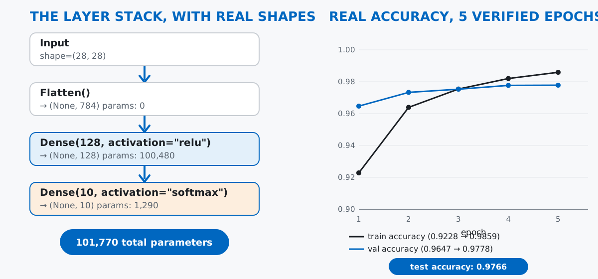

All five of these test images were classified correctly, each with a predicted-class probability above 0.997 — predict() returns the full probability distribution over all 10 digits for every image; argmax here just picks the digit predict() was most confident about.

Four Gotchas Worth Knowing

Skipping normalization doesn’t error — it just trains worse, visibly. Here’s the same architecture, same random seed, trained for 3 epochs on raw 0–255 pixel values instead of the normalized 0–1 ones:

model_unnorm.fit(X_train.astype("float32"), y_train, epochs=3, batch_size=32, validation_split=0.1, verbose=2)

Epoch 1/3
1688/1688 - 2s - 1ms/step - accuracy: 0.8550 - loss: 2.5192 - val_accuracy: 0.9057 - val_loss: 0.4167
Epoch 2/3
1688/1688 - 2s - 1ms/step - accuracy: 0.9100 - loss: 0.3747 - val_accuracy: 0.9318 - val_loss: 0.2859
Epoch 3/3
1688/1688 - 2s - 1ms/step - accuracy: 0.9250 - loss: 0.2940 - val_accuracy: 0.9385 - val_loss: 0.2462

The same architecture on normalized data, same seed, same 3 epochs:

Epoch 1/3
1688/1688 - 2s - 1ms/step - accuracy: 0.9213 - loss: 0.2727 - val_accuracy: 0.9652 - val_loss: 0.1197
Epoch 2/3
1688/1688 - 2s - 1ms/step - accuracy: 0.9646 - loss: 0.1194 - val_accuracy: 0.9710 - val_loss: 0.0958
Epoch 3/3
1688/1688 - 2s - 1ms/step - accuracy: 0.9763 - loss: 0.0812 - val_accuracy: 0.9740 - val_loss: 0.0858

After 3 identical epochs, unnormalized validation accuracy is 0.9385; normalized is already at 0.9740, a gap the unnormalized run never closes in the epochs shown. Unnormalized loss also starts at a startling 2.5192, nearly ten times the normalized run’s 0.2727 — the large raw pixel values push the first gradients to a much larger, less well-behaved scale, exactly as the normalization section predicted.

A falling loss and a rising accuracy are related, but not the same signal, and they don’t move in lockstep. Compare epoch 4 to epoch 5 of the main training run above: loss dropped from 0.0585 to 0.0454, a 22% relative improvement, while accuracy only inched from 0.9820 to 0.9859, a gain of well under half a percentage point. That’s expected, not a bug: accuracy only counts whether the highest-probability class was correct, a blunt yes/no per image. Loss keeps rewarding the model for every fraction of a percent more confidence it puts on the right answer, even on images it was already classifying correctly — so loss can keep improving smoothly long after accuracy has nearly maxed out.

Overfitting is invisible if you only watch training numbers. Train the same architecture on just 500 images (well under 1% of the full training set) for 15 epochs, watching training and validation accuracy separately:

model_tiny.fit(X_tiny, y_tiny, epochs=15, batch_size=32, validation_split=0.2, verbose=2)

Epoch  1: accuracy=0.4450  val_accuracy=0.6900
Epoch  5: accuracy=0.9250  val_accuracy=0.8400
Epoch  8: accuracy=0.9775  val_accuracy=0.8600
Epoch 13: accuracy=1.0000  val_accuracy=0.8400
Epoch 15: accuracy=1.0000  val_accuracy=0.8400

(Full 15-epoch log verified; every 5th epoch shown here for space — see the notes file for the complete run.) Training accuracy climbs all the way to a perfect 1.0000 by epoch 13. Validation accuracy peaks around 0.86 near epoch 8–10 and then drifts back down to 0.84, even as training accuracy keeps looking better and better. A reader who only printed accuracy — not val_accuracy — would see a number that never stops improving and conclude the model is still getting better, right up to memorizing its 500 training images perfectly. The fix isn’t a special function; it’s the same discipline as the honest-quiz mental model from our first machine learning model post — always report the validation or test number, never the training number, when you’re deciding whether a model is actually good.

The first call to fit() or a dataset loader can look slow and noisy — that’s normal, not a failure. tf.keras.datasets.mnist.load_data() in the dataset section above printed a real download progress bar the first time it ran on this machine (MNIST is fetched once and cached locally afterward), and every fit()/evaluate() call prints a per-batch progress indicator with step timing (1ms/step, 508us/step) while it runs. None of that is an error — it’s Keras being verbose about work it’s actually doing. If you see CPU-optimization or hardware-acceleration messages the first time you import tensorflow on your own machine, those are informational too; they’re TensorFlow reporting what hardware path it picked, not a warning that something is broken.

Wrapping Up

The mental model holds regardless of how many layers you stack: transform the input through a chain of learned layers, compare the result to the truth with a loss function, and nudge every weight to make that loss a little smaller, repeated over many epochs. Mapped onto the tools:

• tf.keras.Sequential([...]) → describes the stack of layers, in order, from raw input to final prediction
• Dense(units, activation=...) → one learned transformation, relu in hidden layers, softmax for a multi-class output
• model.compile(optimizer, loss, metrics) → sets how wrongness is measured, how weights get nudged, and what to report
• model.fit(X, y, epochs=...) → runs the actual training loop, one epoch at a time, printing loss and accuracy for both training and validation data
• model.evaluate(X_test, y_test) → the one honest number that matters, computed on data the model never trained or validated on
• normalized inputs → not optional for stable, fast training, unlike some of the scaling tradeoffs in scikit-learn models

If you want to go deeper than one small dense network — the math behind backpropagation, multi-layer architectures, and the Keras functional API for more complex models — the Building a Shallow Neural Network with the Sequential API and Introduction to Neural Networks lessons in our free Machine Learning course pick up exactly where this post leaves off.