K-Nearest Neighbors in Python: How the Algorithm Actually Works

“How many of my nearest neighbors agree with me?” is a question you can ask about almost any labeled data, and it turns out to be a complete machine learning algorithm on its own. No formula to fit, no gradient to descend — just distance and a vote. That’s K-Nearest Neighbors (KNN), and it’s one of the few algorithms whose name is also an accurate description of how it works.

If you haven’t seen scikit-learn’s general fit/predict pattern yet, start with our scikit-learn overview — it uses KNeighborsClassifier as one stop on a wider tour of the Estimator API, but never explains what’s actually happening inside .fit() and .predict(). This post goes deep on exactly that one algorithm: what “training” does (spoiler: almost nothing), how the number of neighbors you choose reshapes every prediction, why this particular family of algorithms cares so much about feature scale, and how to pick a good k instead of guessing.

The Mental Model: Store the Data, Decide Later

Most estimators spend their .fit() call doing real work — a linear regression solves for coefficients, a logistic regression runs an optimization loop. KNeighborsClassifier skips all of that. Its mental model is two steps, and the split between them is the whole point:

1. .fit(X, y) just stores the training data. No coefficients are learned, no loss function is minimized. The “model” after fitting is, essentially, the training set itself, lightly indexed for faster lookups.
2. .predict(x) does all the actual work, for every single query. Given a new point, KNN measures the distance from that point to every stored training point, keeps the k closest ones, and lets them vote. For classification, the majority class among those k neighbors wins. For regression, it’s the average of their target values instead of a vote.

That’s the entire algorithm. There’s no equation to memorize because there isn’t really a fitted equation at all — just “find who’s nearby, and copy them.”

A naming note worth clearing up here: K-Nearest Neighbors is not the same algorithm as K-Means, even though the names and the letter k invite confusion. Our post on dominant colors with K-Means covers K-Means clustering, which is unsupervised — it has no labels at all, and it invents groups by moving cluster centers around. KNN is the opposite: it’s supervised, every training point already has a known label, and there are no cluster centers to compute. The only thing the two algorithms share is that both measure distance between points and both have a parameter called k. Past that, they solve different problems.

A Dataset You Can Reproduce

Rather than downloading anything, we’ll use a dataset that ships with scikit-learn itself, so your numbers will match mine exactly with nothing more than pip install scikit-learn. Imagine you work with a small diagnostic lab: a set of cell-nuclei measurements has been extracted from breast-mass biopsy images, and you want a model that flags which samples look malignant from the measurements alone, before a pathologist’s final read.

Data: the Breast Cancer Wisconsin (Diagnostic) dataset bundled with scikit-learn (originally donated to the UCI Machine Learning Repository by the University of Wisconsin; public research data, redistributed under scikit-learn’s BSD license), loaded via load_breast_cancer().

import pandas as pd
from sklearn.datasets import load_breast_cancer

cancer = load_breast_cancer(as_frame=True)
df = cancer.frame
df[["mean radius", "mean texture", "mean area", "mean smoothness", "target"]].head()

   mean radius  mean texture  mean area  mean smoothness  target
0        17.99         10.38     1001.0          0.11840       0
1        20.57         17.77     1326.0          0.08474       0
2        19.69         21.25     1203.0          0.10960       0
3        11.42         20.38      386.1          0.14250       0
4        20.29         14.34     1297.0          0.10030       0

df.shape

(569, 31)

569 samples, 30 numeric measurements, and one target column. (The outputs in this post come from pandas 3.0 and scikit-learn 1.9.)

df["target"].value_counts().sort_index()
print(cancer.target_names)

target
0    212
1    357
Name: count, dtype: int64
['malignant' 'benign']

0 means malignant, 1 means benign — 212 malignant and 357 benign samples, close enough to balanced that plain accuracy is a fair headline metric later on.

Fitting a KNeighborsClassifier

Set aside a test set the model never sees during “training” — the same discipline every supervised model needs, KNN included, even though its training step barely does anything:

from sklearn.model_selection import train_test_split
from sklearn.neighbors import KNeighborsClassifier
from sklearn.metrics import accuracy_score

X = df.drop(columns=["target"])
y = df["target"]
X_train, X_test, y_train, y_test = train_test_split(
    X, y, test_size=0.2, random_state=42, stratify=y
)
X_train.shape, X_test.shape

((455, 30), (114, 30))

stratify=y keeps the same malignant/benign proportions in both slices. Now configure and fit — full detail on every constructor argument lives in scikit-learn’s KNeighborsClassifier reference:

knn = KNeighborsClassifier(n_neighbors=5)
knn.fit(X_train, y_train)
y_pred = knn.predict(X_test)

preview = pd.DataFrame({"actual": y_test.values[:5], "predicted": y_pred[:5]})
preview

   actual  predicted
0       0          0
1       1          1
2       0          0
3       1          0
4       0          0

acc_baseline = accuracy_score(y_test, y_pred)
print(f"accuracy (k=5, unscaled, all 30 features): {acc_baseline:.3f}")

accuracy (k=5, unscaled, all 30 features): 0.912

Four of five preview rows match, and 91.2% overall. That .fit() call above didn’t learn anything in the usual sense — it stored 455 rows. Every one of those correct-or-wrong predictions was decided at .predict() time, by measuring distance to those 455 stored points.

What Changing k Does to the Decision Boundary

To actually see what k controls, it helps to drop down to two features you can plot on a page. mean radius (tumor size) correlates strongly with the diagnosis; mean texture (variation in grayscale values across the cell image) is a much weaker signal on its own, but the two together are easy to reason about and visually intuitive, even though they’re not the two most predictive columns in the dataset:

corrs = df.corr(numeric_only=True)["target"].abs().sort_values(ascending=False)
print(f"mean radius correlation with target: {corrs['mean radius']:.3f}")
print(f"mean texture correlation with target: {corrs['mean texture']:.3f} (rank {list(corrs.index).index('mean texture')} of 30)")

mean radius correlation with target: 0.730
mean texture correlation with target: 0.415 (rank 19 of 30)

feat1, feat2 = "mean radius", "mean texture"
X2 = df[[feat1, feat2]].to_numpy()
X2_train, X2_test, y2_train, y2_test = train_test_split(
    X2, y, test_size=0.2, random_state=42, stratify=y
)

Now fit the same classifier at a few different k values and watch accuracy move:

for k in [1, 5, 15, 51]:
    m = KNeighborsClassifier(n_neighbors=k)
    m.fit(X2_train, y2_train)
    acc = accuracy_score(y2_test, m.predict(X2_test))
    print(f"k={k:>3}: accuracy={acc:.3f}")

k=  1: accuracy=0.842
k=  5: accuracy=0.868
k= 15: accuracy=0.877
k= 51: accuracy=0.895

Small k means each prediction depends on a handful of nearby points, so the decision boundary can bend sharply around individual samples — including noisy or mislabeled ones, which is why k=1 scores lowest here. Larger k averages over more neighbors, smoothing the boundary into broader regions, which is why accuracy climbs as k grows on just these two features. That trend doesn’t continue forever (an extremely large k eventually just predicts the majority class everywhere), but in this range, more voters means less noise.

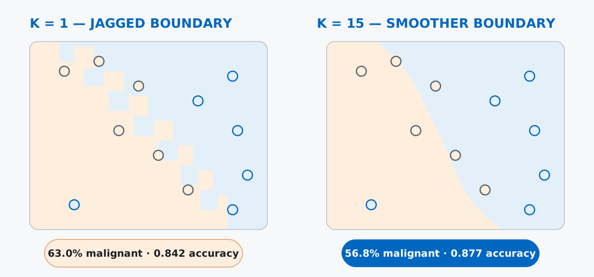
At k=1, the boundary between the malignant and benign regions follows every single training point, carving out small malignant-labeled islands inside mostly-benign territory. At k=15, those islands mostly disappear — the boundary follows the general shape of the two classes instead of any one point’s exact location.

Why Feature Scaling Matters for a Distance-Based Model

Switch back to all 30 features, unscaled, and something is being left on the table:

from sklearn.preprocessing import StandardScaler

acc_unscaled = accuracy_score(y_test, knn.predict(X_test))
print(f"accuracy (unscaled, k=5): {acc_unscaled:.3f}")

scaler = StandardScaler()
X_train_scaled = scaler.fit_transform(X_train)
X_test_scaled = scaler.transform(X_test)

knn_scaled = KNeighborsClassifier(n_neighbors=5)
knn_scaled.fit(X_train_scaled, y_train)
acc_scaled = accuracy_score(y_test, knn_scaled.predict(X_test_scaled))
print(f"accuracy (scaled, k=5): {acc_scaled:.3f}")

accuracy (unscaled, k=5): 0.912
accuracy (scaled, k=5): 0.956

0.912 to 0.956 — scaling alone fixed roughly 5 more predictions out of 114. This isn’t the usual “always scale your features” advice; it’s specific to how KNN decides what “nearest” means. Every other algorithm you’ve probably used learns weights that can, in principle, compensate for a feature living on a huge scale. KNN has no weights to learn — distance is computed directly on the raw numbers, so whichever feature happens to have the largest numeric range automatically dominates:

print(X_train[["mean area", "mean smoothness"]].std().round(3))
ratio = X_train["mean area"].std() / X_train["mean smoothness"].std()
print(f"mean area's std is {ratio:,.0f}x mean smoothness's std")

mean area          344.945
mean smoothness      0.013
dtype: float64
mean area's std is 25,632x mean smoothness's std

mean area is measured in square pixels and runs into the thousands; mean smoothness is a ratio that stays under 0.2. Plug both into the same Euclidean distance formula and see what happens to two real training rows:

r1, r2 = X_train.iloc[0], X_train.iloc[1]
d_area = (r1["mean area"] - r2["mean area"]) ** 2
d_smooth = (r1["mean smoothness"] - r2["mean smoothness"]) ** 2
share = d_area / (d_area + d_smooth) * 100
print(f"squared difference in mean area: {d_area:,.1f}")
print(f"squared difference in mean smoothness: {d_smooth:.6f}")
print(f"mean area alone accounts for {share:.4f}% of their combined squared distance")

squared difference in mean area: 855,810.0
squared difference in mean smoothness: 0.000359
mean area alone accounts for 100.0000% of their combined squared distance

Between just these two columns, mean smoothness contributes essentially nothing to “how far apart” these two patients are, even though a doctor might consider it just as diagnostically relevant. StandardScaler fixes this by rescaling every feature to the same mean-0, standard-deviation-1 footing before distance is ever computed, which is exactly why the scaled model’s accuracy jumped.

Choosing k Systematically

Nothing so far justifies why k=5 was a reasonable starting point — it wasn’t tuned, just a common default. A simple loop over candidate values, checked against a validation split carved out of the training data (never the test set), finds a better one:

X_train_sub, X_val, y_train_sub, y_val = train_test_split(
    X_train_scaled, y_train, test_size=0.25, random_state=42, stratify=y_train
)

val_scores = {}
for k in range(1, 26, 2):
    m = KNeighborsClassifier(n_neighbors=k)
    m.fit(X_train_sub, y_train_sub)
    acc = accuracy_score(y_val, m.predict(X_val))
    val_scores[k] = acc
    print(f"k={k:>2}: validation accuracy={acc:.4f}")

best_k = max(val_scores, key=val_scores.get)
print(f"best k on validation set: {best_k} (accuracy={val_scores[best_k]:.4f})")

k= 1: validation accuracy=0.9386
k= 3: validation accuracy=0.9649
k= 5: validation accuracy=0.9649
k= 7: validation accuracy=0.9649
k= 9: validation accuracy=0.9474
k=11: validation accuracy=0.9386
k=13: validation accuracy=0.9386
k=15: validation accuracy=0.9386
k=17: validation accuracy=0.9386
k=19: validation accuracy=0.9386
k=21: validation accuracy=0.9298
k=23: validation accuracy=0.9298
k=25: validation accuracy=0.9298

Only odd values of k were tried here on purpose — more on why in the gotchas section below. Accuracy peaks in a plateau from k=3 to k=7 and drifts downward afterward; max() with ties keeps the first, so best_k lands on 3. Refit on the full training set at that k and check the number that actually matters, the held-out test accuracy:

final_knn = KNeighborsClassifier(n_neighbors=best_k)
final_knn.fit(X_train_scaled, y_train)
final_acc = accuracy_score(y_test, final_knn.predict(X_test_scaled))
print(f"held-out test accuracy with k={best_k}: {final_acc:.3f}")

held-out test accuracy with k=3: 0.982

98.2%, up from 91.2% at the unscaled, untuned k=5 we started with — scaling and a properly chosen k accounted for almost all of that gain.

KNN for Regression, Briefly

Everything above used KNeighborsClassifier, which votes on a class. KNeighborsRegressor follows the identical mental model — store the data, find the k nearest neighbors at prediction time — but averages their target values instead of voting on a label:

import numpy as np
from sklearn.neighbors import KNeighborsRegressor

rng = np.random.default_rng(42)
x_reg = np.sort(rng.uniform(0, 10, size=30))
y_reg = np.sin(x_reg) + rng.normal(0, 0.15, size=30)
X_reg = x_reg.reshape(-1, 1)

reg = KNeighborsRegressor(n_neighbors=3)
reg.fit(X_reg, y_reg)

query = np.array([[5.0]])
dist, idx = reg.kneighbors(query)
print("query x = 5.0")
print("3 nearest x values:", x_reg[idx[0]].round(2))
print("3 nearest y values:", y_reg[idx[0]].round(3))
print("predicted y (mean of the 3 neighbors' y values):", reg.predict(query)[0].round(3))

query x = 5.0
3 nearest x values: [4.67 4.5  5.55]
3 nearest y values: [-1.099 -0.897 -0.637]
predicted y (mean of the 3 neighbors' y values): -0.878

-0.878 is the plain mean of [-1.099, -0.897, -0.637] — nothing more sophisticated is happening. Same algorithm, same lookup, just mean() instead of a majority vote at the end.

Three Gotchas Worth Knowing

An even k can produce an exact tie in binary classification, and scikit-learn breaks it silently. With two classes, an even number of neighbors can split right down the middle. It’s not a theoretical risk — it happens in this exact dataset:

m2 = KNeighborsClassifier(n_neighbors=2)
m2.fit(X2_train, y2_train)
proba2 = m2.predict_proba(X2_test)
for i, p in enumerate(proba2):
    if abs(p[0] - 0.5) < 1e-9:
        dist, idx = m2.kneighbors(X2_test[i:i + 1])
        print("tied test point (mean radius, mean texture):", X2_test[i])
        print("distances to its 2 nearest neighbors:", dist[0].round(3))
        print("classes of its 2 nearest neighbors:", y2_train.to_numpy()[idx[0]])
        print("predict_proba:", p)
        print("predicted class (scikit-learn's tie-break):", m2.predict(X2_test[i:i + 1])[0])
        break

tied test point (mean radius, mean texture): [14.45 20.22]
distances to its 2 nearest neighbors: [0.247 0.398]
classes of its 2 nearest neighbors: [0 1]
predict_proba: [0.5 0.5]
predicted class (scikit-learn's tie-break): 0

This test point’s two nearest neighbors are one malignant, one benign — a genuine 50/50 vote. scikit-learn doesn’t raise an error or flag it; predict() just returns a class anyway (here, the lower-numbered one). Use an odd k for two-class problems so a tie like this can’t happen in the first place — which is exactly why the systematic sweep above only tried odd values.

There’s no free lunch from skipping the training step — the cost just moves to every prediction. Because .fit() does almost no work, .predict() has to scan the stored training set every single time it’s called, and that cost scales with how much data you’ve stored:

import time
from sklearn.linear_model import LogisticRegression

rng2 = np.random.default_rng(0)
X_query = rng2.normal(size=(500, 10))
for n in [1000, 10000, 100000]:
    Xt = rng2.normal(size=(n, 10))
    yt = rng2.integers(0, 2, size=n)

    m = KNeighborsClassifier(n_neighbors=5)
    m.fit(Xt, yt)
    t0 = time.perf_counter()
    m.predict(X_query)
    knn_t = time.perf_counter() - t0

    lr = LogisticRegression(max_iter=200)
    lr.fit(Xt, yt)
    t0 = time.perf_counter()
    lr.predict(X_query)
    lr_t = time.perf_counter() - t0

    print(f"n_train={n:>7,}: KNeighborsClassifier.predict(500)={knn_t*1000:6.2f}ms   LogisticRegression.predict(500)={lr_t*1000:6.2f}ms")

n_train=  1,000: KNeighborsClassifier.predict(500)=  6.54ms   LogisticRegression.predict(500)=  0.15ms
n_train= 10,000: KNeighborsClassifier.predict(500)= 36.01ms   LogisticRegression.predict(500)=  0.17ms
n_train=100,000: KNeighborsClassifier.predict(500)=115.35ms   LogisticRegression.predict(500)=  0.21ms

LogisticRegression pays its cost once, upfront, during .fit() — after that, predicting is just a fixed-size dot product no matter how much training data it saw, so its predict time barely moves. KNeighborsClassifier’s predict time climbs roughly in step with the training-set size, because it’s re-scanning the stored data on every call. For a small teaching dataset like ours, that’s invisible. For a production system scoring millions of rows against a large stored dataset, it’s a real operational cost.

Forgetting to scale new data the same way you scaled the training data fails silently, not loudly. This is a different mistake from not scaling at all — it’s scaling inconsistently between fit and predict:

acc_correct = accuracy_score(y_test, knn_scaled.predict(X_test_scaled))
print(f"predict on properly scaled X_test:  accuracy={acc_correct:.3f}")

acc_bug = accuracy_score(y_test, knn_scaled.predict(X_test))
print(f"predict on raw, UNSCALED X_test:    accuracy={acc_bug:.3f}")

/.../sklearn/utils/validation.py:2820: UserWarning: X has feature names, but KNeighborsClassifier was fitted without feature names
  warnings.warn(
predict on properly scaled X_test:  accuracy=0.956
predict on raw, UNSCALED X_test:    accuracy=0.368

knn_scaled was fitted on scaled data; handing it X_test in its raw, unscaled form doesn’t raise a scaling error — scikit-learn only warns about missing column names, which is a red herring here. The real damage is silent: accuracy collapses from 0.956 to 0.368, worse than always guessing the majority class would score. Every distance calculation is still technically valid arithmetic, it’s just comparing numbers on the wrong scale. Fit the scaler once, and apply that exact same fitted scaler.transform() call everywhere the model is used, training and prediction alike.

Wrapping Up

One mental model covers the whole algorithm:

• .fit(X, y) → stores the training data, does essentially no computation
• .predict(x) → measures distance to every stored point, keeps the k closest, and votes (classification) or averages (regression)
• Small k → boundary follows individual points closely, more sensitive to noise
• Large k → boundary smooths out, more resistant to noise but less locally precise
• StandardScaler → essential before fitting, since raw distance calculations let large-magnitude features silently dominate
• Odd k → avoids exact vote ties in two-class problems

If you want a guided, from-scratch build of this exact algorithm — including how the vote and the distance metric work step by step — the Introduction to K-Nearest Neighbors lesson in our free Machine Learning course is the natural next stop, and its guided project on predicting breast cancer diagnosis picks up on the exact dataset used in this post.