Linear Regression in Python: Fitting a Line and Reading the Coefficients

LinearRegression().fit(X, y) runs in a fraction of a second, prints nothing alarming, and hands you back a coef_ array. It’s easy to stop right there and treat the number as done. Our post on training your first machine learning model uses that exact class as its running example, but it stays at the workflow level — split, fit, predict, grade — and never opens up what the fitted coefficients themselves are saying. This post does that: what a coefficient means, how confident you should be in it, and where that confidence quietly breaks down.

Concretely: model.coef_[i] is how much the target changes for a one-unit increase in feature i, holding every other feature fixed, and model.intercept_ is the predicted value when every feature is zero. scikit-learn stops there — it never tells you whether a coefficient is distinguishable from zero. For that you fit the same data again with statsmodels.api.OLS, whose .summary() reports a standard error, a p-value, and a confidence interval for every coefficient. Both libraries fit the identical line — ordinary least squares, minimizing the sum of squared residuals — they just report different things about it.

One Line, Minimizing Squared Error

Every linear regression, whether it has one feature or fifty, is a weighted sum: multiply each feature by a coefficient, add an intercept, and that sum is the prediction. Fitting the model means choosing the coefficients and intercept that make the predictions as close to the real targets as possible — specifically, the choice that minimizes the sum of squared differences between predicted and actual values across every row. That’s the “least squares” in ordinary least squares, and it’s the same objective whether scikit-learn solves it with a direct linear-algebra computation or statsmodels solves it the same way under a different API.

Two things follow from that objective. First, “closer on average” isn’t the same as “correct for every point” — a straight line is a compromise, and some rows will sit well off it no matter how good the fit is. Second, squaring the errors means large misses count disproportionately more than small ones, which is why one wildly wrong row can pull a fitted line further than several ordinary ones — worth remembering later, when a coefficient looks larger or smaller than intuition suggests.

398 Cars and Their Fuel Economy

Data: the Auto MPG dataset, originally collected for a 1983 American Statistical Association exposition and hosted at the UCI Machine Learning Repository (CC BY 4.0). It’s 398 US and international cars from the 1970s and early 1980s, with fuel economy and a handful of physical specs for each one — exactly the shape linear regression was built for: several continuous predictors, one continuous target.

import pandas as pd

cars = pd.read_csv("auto-mpg.csv", na_values="?")
cars.shape

(398, 9)

cars[["mpg", "weight", "horsepower", "model_year", "car_name"]].head()

    mpg  weight  horsepower  model_year                   car_name
0  18.0    3504       130.0          70  chevrolet chevelle malibu
1  15.0    3693       165.0          70          buick skylark 320
2  18.0    3436       150.0          70         plymouth satellite
3  16.0    3433       150.0          70              amc rebel sst
4  17.0    3449       140.0          70                ford torino

weight is in pounds and model_year is the last two digits of the year (70 means 1970), the dataset’s own original units — no conversion here, so the coefficients later stay in units you can sanity-check by eye. (The outputs in this post come from pandas 3.0, scikit-learn 1.9, and statsmodels 0.14 — everything shown also works on pandas 2.x.) One column needs attention before anything gets fit:

cars.isna().sum()

mpg             0
cylinders       0
displacement    0
horsepower      6
weight          0
acceleration    0
model_year      0
origin          0
car_name        0
dtype: int64

Six cars are missing horsepower — the original 1983 dataset just never recorded it for those rows. Loading with na_values="?" turns the source file’s literal ? placeholder into a real, visible NaN instead of a string that would silently break any arithmetic on the column.

A Regression Line, One Feature at a Time

Start with the feature most people would guess matters most: a heavier car should get worse mileage.

from sklearn.linear_model import LinearRegression

simple_model = LinearRegression()
simple_model.fit(cars[["weight"]], cars["mpg"])
print(simple_model.coef_, simple_model.intercept_)

[-0.00767661] 46.31736442026565

Read the coefficient in the feature’s own units: every additional pound of weight is associated with about 0.0077 fewer miles per gallon. That’s small-sounding on its own, but weight in this dataset ranges from 1,613 to 5,140 pounds — a roughly 3,500-pound spread — so the model’s predicted mileage moves by more than 26 mpg from the lightest car to the heaviest, holding nothing else fixed because nothing else is in the model yet. The intercept, 46.3, is the predicted mpg for a (hypothetical, nonexistent) car that weighs nothing — mathematically necessary, not a number to read literally.

from sklearn.metrics import r2_score

r2_score(cars["mpg"], simple_model.predict(cars[["weight"]]))

0.6917929800341573

Weight alone explains about 69% of the variance in mpg across all 398 cars.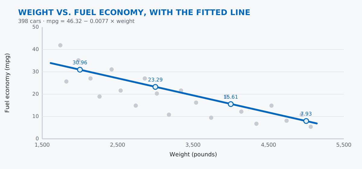

weights = pd.DataFrame({"weight": [2000, 3000, 4000, 5000]})
simple_model.predict(weights).round(2)

[30.96 23.29 15.61  7.93]

Each extra 1,000 pounds costs almost exactly 7.7 mpg in this model — the coefficient times 1,000, restated as a round number that’s easier to hold in your head.

Adding More Features

A car’s mileage isn’t only about weight. Add horsepower, displacement (engine size), acceleration, and model year, and fit again:

features = ["weight", "horsepower", "displacement", "acceleration", "model_year"]
print(cars.shape[0], cars.dropna(subset=features).shape[0])

398 392

dropna just quietly removed the six cars with missing horsepower — worth checking the row count before and after any time you drop rows, since it’s easy to lose more of your sample than you meant to without a single warning.

clean = cars.dropna(subset=features).copy()

multi_model = LinearRegression()
multi_model.fit(clean[features], clean["mpg"])

pd.Series(multi_model.coef_, index=features).round(4)

weight         -0.0069
horsepower      0.0010
displacement    0.0028
acceleration    0.0903
model_year      0.7541
dtype: float64

from sklearn.metrics import mean_absolute_error

preds = multi_model.predict(clean[features])
print("intercept:", round(multi_model.intercept_, 2))
print("R2:", round(r2_score(clean["mpg"], preds), 4))
print("MAE:", round(mean_absolute_error(clean["mpg"], preds), 2))

intercept: -15.44
R2: 0.8088
MAE: 2.62

R² climbed from 0.69 to 0.81 with the extra features, and the average prediction is now off by 2.62 mpg. Notice weight’s coefficient barely moved (-0.0077 alone, -0.0069 here) — a good sign it’s capturing something real about weight specifically, not just standing in for the other specs. model_year’s coefficient, 0.75, says each model year later is worth about three-quarters of an mpg on average, which matches the real story of 1970s fuel-efficiency regulation pushing engines to improve year over year.

The Numbers scikit-learn Doesn’t Show You

Every coefficient above is a single number with no sense of how confident the model is in it. statsmodels’ OLS fits the identical line and reports a standard error, a t-statistic, a p-value, and a 95% confidence interval alongside each one:

import statsmodels.api as sm

X = sm.add_constant(clean[features])
ols_model = sm.OLS(clean["mpg"], X).fit()
print(ols_model.summary())

                            OLS Regression Results                            
==============================================================================
Dep. Variable:                    mpg   R-squared:                       0.809
Model:                            OLS   Adj. R-squared:                  0.806
Method:                 Least Squares   F-statistic:                     326.5
Date:                Sat, 18 Jul 2026   Prob (F-statistic):          3.26e-136
Time:                        09:21:31   Log-Likelihood:                -1037.0
No. Observations:                 392   AIC:                             2086.
Df Residuals:                     386   BIC:                             2110.
Df Model:                           5                                         
Covariance Type:            nonrobust                                         
================================================================================
                   coef    std err          t      P>|t|      [0.025      0.975]
--------------------------------------------------------------------------------
const          -15.4353      4.677     -3.300      0.001     -24.631      -6.240
weight          -0.0069      0.001    -10.333      0.000      -0.008      -0.006
horsepower       0.0010      0.014      0.074      0.941      -0.026       0.028
displacement     0.0028      0.005      0.509      0.611      -0.008       0.014
acceleration     0.0903      0.102      0.886      0.376      -0.110       0.291
model_year       0.7541      0.053     14.334      0.000       0.651       0.858
==============================================================================
Omnibus:                       37.089   Durbin-Watson:                   1.224
Prob(Omnibus):                  0.000   Jarque-Bera (JB):               57.937
Skew:                           0.626   Prob(JB):                     2.63e-13
Kurtosis:                       4.407   Cond. No.                     8.37e+04
==============================================================================

Notes:
[1] Standard Errors assume that the covariance matrix of the errors is correctly specified.
[2] The condition number is large, 8.37e+04. This might indicate that there are
strong multicollinearity or other numerical problems.

The coef column matches scikit-learn’s coef_ exactly — same model, same math. What’s new is P>|t|: weight and model_year have p-values under 0.001, meaning the data is very unlikely to look this way if those coefficients were really zero. horsepower, displacement, and acceleration all have p-values well above the usual 0.05 cutoff — 0.941, 0.611, and 0.376. Taken at face value, that says the model can’t distinguish their effect from zero once weight and model year are already in it. Statsmodels even flags the likely reason at the bottom: “strong multicollinearity or other numerical problems.” Worth chasing down before believing it.

When Coefficients Start Leaning on Each Other

Multicollinearity means two or more features are themselves strongly correlated, so the model can’t cleanly separate “this is what weight does” from “this is what displacement does” — it just knows their combination predicts mpg well, and the individual coefficients and their standard errors get unstable. Check pairwise correlation first:

clean[features].corr().round(3)

              weight  horsepower  displacement  acceleration  model_year
weight         1.000       0.865         0.933        -0.417      -0.309
horsepower     0.865       1.000         0.897        -0.689      -0.416
displacement   0.933       0.897         1.000        -0.544      -0.370
acceleration  -0.417      -0.689        -0.544         1.000       0.290
model_year    -0.309      -0.416        -0.370         0.290       1.000

Weight, horsepower, and displacement are all correlated with each other above 0.86 — a bigger engine tends to mean a heavier, more powerful car, which is exactly the redundancy that confuses a regression’s coefficients. Variance inflation factor (VIF) turns that into one number per feature, but it’s easy to compute wrong. Calling it on the raw feature matrix, without a constant column, is the mistake most people make first:

from statsmodels.stats.outliers_influence import variance_inflation_factor

pd.Series(
    [variance_inflation_factor(clean[features].values, i) for i in range(len(features))],
    index=features,
).round(1)

weight          136.5
horsepower       60.2
displacement     48.3
acceleration     69.3
model_year       96.0
dtype: float64

Those numbers are wildly inflated — variance_inflation_factor assumes an intercept is already part of what it’s regressing against, and without one it’s effectively measuring variance around zero instead of around the mean. Pass it the same constant-added matrix OLS used, and the picture becomes far more reasonable (ignore the const row itself — it isn’t a real predictor):

vif = pd.Series(
    [variance_inflation_factor(X.values, i) for i in range(X.shape[1])],
    index=X.columns,
).round(1)
vif

const           726.6
weight           10.6
horsepower        9.3
displacement     10.8
acceleration      2.6
model_year        1.2
dtype: float64

A VIF above 10 is the commonly cited danger line, meaning that feature’s variance is more than ten times what it would be if it were uncorrelated with the others. weight (10.6) and displacement (10.8) both cross it, and horsepower (9.3) sits right at the edge — matching the correlation matrix and matching exactly the three features whose p-values collapsed above. acceleration (2.6) and model_year (1.2) are fine; that’s why their coefficients stayed sharp and significant.

Comparing Coefficients Fairly

Look back at the raw coefficients — model_year at 0.75 versus weight at -0.0069 — and it’s tempting to read model_year as the more important feature just because its number is bigger. That’s a scale illusion: model_year moves in units of one year, weight moves in units of one pound. Standardizing every feature to a common scale (mean zero, one standard deviation wide) before fitting makes the coefficients directly comparable in “effect per one standard deviation of the feature”:

X_std = (clean[features] - clean[features].mean()) / clean[features].std()

std_model = LinearRegression()
std_model.fit(X_std, clean["mpg"])
pd.Series(std_model.coef_, index=features).round(2)

weight         -5.84
horsepower      0.04
displacement    0.29
acceleration    0.25
model_year      2.78
dtype: float64

On this fair footing, weight (-5.84) is clearly the dominant predictor, model_year (2.78) second — the opposite conclusion from eyeballing the raw coefficients, where model_year’s 0.75 looked bigger than weight’s -0.0069. The Interpreting Regression Parameters lesson in our Machine Learning course builds this same standardization idea further on a different car dataset, if you want more practice with it.

Checking That the Line Actually Fits

R² and p-values both assume the true relationship is a straight line in the first place. Nothing checked that assumption yet. Split the simple weight-only model’s errors — its residuals — by weight range and see if they average to zero everywhere, or drift:

cars["pred_mpg"] = simple_model.predict(cars[["weight"]])
cars["resid"] = cars["mpg"] - cars["pred_mpg"]
cars["weight_group"] = pd.qcut(cars["weight"], q=3, labels=["Light", "Mid", "Heavy"])

cars.groupby("weight_group", observed=True)["resid"].mean().round(2)

weight_group
Light    0.89
Mid     -1.04
Heavy    0.13
Name: resid, dtype: float64

A truly straight-line relationship would leave those three averages close to zero and patternless. Instead they dip from positive to negative and back to positive — the straight line is a little too flat in the middle of the weight range and a little too steep at the extremes, a real (if modest) curve the line can’t bend to follow. Adding a squared weight term confirms it:

cars["weight_sq"] = cars["weight"] ** 2

quad_model = LinearRegression()
quad_model.fit(cars[["weight", "weight_sq"]], cars["mpg"])
quad_preds = quad_model.predict(cars[["weight", "weight_sq"]])

print("linear R2:   ", round(r2_score(cars["mpg"], cars["pred_mpg"]), 4))
print("quadratic R2:", round(r2_score(cars["mpg"], quad_preds), 4))

linear R2:    0.6918
quadratic R2: 0.7148

A real, if modest, improvement — 0.6918 up to 0.7148 — from letting the fit curve instead of forcing a straight line, which is exactly what the tercile pattern predicted before either model was refit.

That leaves one honest caveat about the significance section above: a p-value over 0.05 means “not distinguishable from zero given this model and this data,” not “this feature doesn’t matter to fuel economy.” Horsepower obviously affects how a car burns fuel — it’s just that once weight and displacement are already in the model, there’s too little independent horsepower signal left for the regression to pin down cleanly. Dropping a feature because of a high p-value, without first checking whether multicollinearity is the actual cause, throws away information the model never got a fair chance to use.

If you want to keep building on this — comparing models honestly with a held-out test set, or moving from a continuous target to a category — the Regression module in our free Machine Learning course covers gradient descent and a guided insurance-cost project, and our post on logistic regression picks up the same coefficient-interpretation habit for a yes-or-no target instead of a number.