Logistic Regression in Python: Sigmoid, Odds Ratios, and Thresholds

Some questions have a yes-or-no answer: will this patient develop diabetes, is this transaction fraudulent, will a customer churn. You’ve got a table of features and a category to predict, not a number to forecast — and that distinction matters more than it sounds like it should. Our post on training your first machine learning model fits a LinearRegression model that predicts a disease-progression score anywhere on a continuous scale; nothing in that model’s math keeps its output between 0 and 1, because nothing about it is trying to. Logistic regression is the tool built for exactly that constraint — a category, expressed honestly as a probability first.

The name is confusing on purpose: it’s still, underneath, a regression — a line fit through your features, with one learned weight per feature. The twist is what happens to that line before it becomes a prediction, and that’s also where people quietly lose the thread, calling .fit() and .predict() without ever seeing what the fitted numbers actually mean. (If you’ve already met LogisticRegression in passing — our scikit-learn overview uses KNeighborsClassifier as its running example, but name-drops logistic regression as the next stop — this is that deep dive: what’s happening inside .fit(), what the coefficients say, and how to grade the result honestly.) This post builds the mental model first, then works a real binary classification problem end to end: fit the model, read its probabilities, interpret its coefficients, and evaluate it properly.

The Mental Model: A Line Bent Into a Probability

Every linear model, logistic regression included, starts the same way: multiply each feature by a learned weight, add a learned intercept, and sum it up. Call that sum z — it’s the same “weighted combination of features” idea LinearRegression uses, nothing new yet.

In plain linear regression, z is the prediction: a raw number that lands wherever the arithmetic sends it, which is exactly right when the target is something like a disease-progression score. Logistic regression asks a different question and needs one more step to answer it honestly:

1. Compute the same linear combination, z, from the features and the fitted weights.
2. Feed z through the sigmoid function, p = 1 / (1 + e^-z). Whatever z is — a large positive number, a large negative one, exactly zero — sigmoid always returns something between 0 and 1.
3. Read p as a probability: the model’s estimate of “how likely is the positive class,” given this row’s features.
4. Pick a threshold (0.5 by default, not mandatory — more on that later) and turn the probability into a label: p at or above the threshold predicts the positive class, below it predicts the negative one.

That’s the whole idea: logistic regression is a linear model wearing an S-shaped curve as its last step. Sigmoid is monotonic — a bigger z always means a bigger p — so none of z’s straight-line relationship with the features is lost. It’s just recalibrated onto a scale you can honestly call a probability and safely cut into a class.

It’s worth being explicit about how this differs from the other two models this site has already covered. LinearRegression stops at z — no sigmoid, no threshold, because its target genuinely is a continuous number with no upper or lower bound to respect. K-Nearest Neighbors sits at the opposite extreme: it has no z at all. KNeighborsClassifier.fit() doesn’t learn any weights or intercept — it just stores the training rows and does all its real work at prediction time, measuring distance and taking a vote. Logistic regression is the middle case: an explicit, parametric model like linear regression, with coefficients you can read, question, and interpret one by one — but an output that’s a calibrated probability and a class, like KNN’s.

A Dataset You Can Reproduce

This post uses the Pima Indians Diabetes dataset: 768 patient records with eight routine clinical measurements — number of pregnancies, plasma glucose, blood pressure, skin-fold thickness, serum insulin, BMI, a diabetes pedigree function (a score summarizing family history), and age — plus a binary Outcome column: whether that patient was diagnosed with diabetes within five years of the exam. Imagine you work with a small primary-care practice that wants a quick, defensible screening signal from measurements already in a patient’s chart, before ordering the slower and more expensive lab-confirmed test.

Data: the Pima Indians Diabetes dataset, originally collected by the National Institute of Diabetes and Digestive and Kidney Diseases and distributed as CC0 (public domain) via Kaggle’s uciml/pima-indians-diabetes-database, vendored here as a plain CSV at /datasets/blog/logistic-regression-in-python/diabetes.csv.

import pandas as pd

diabetes = pd.read_csv(
    "https://datatweets.com/datasets/blog/logistic-regression-in-python/diabetes.csv"
)
diabetes[["Pregnancies", "Glucose", "BMI", "Age", "Outcome"]].head()

   Pregnancies  Glucose   BMI  Age  Outcome
0            6      148  33.6   50        1
1            1       85  26.6   31        0
2            8      183  23.3   32        1
3            1       89  28.1   21        0
4            0      137  43.1   33        1

diabetes.shape

(768, 9)

diabetes["Outcome"].value_counts()

Outcome
0    500
1    268
Name: count, dtype: int64

768 patients, 8 features, and a target that’s 1 (diabetic) for about 35% of rows and 0 (not diabetic) for the rest — not a rare-event problem, but not perfectly balanced either. Keep that imbalance in mind; it becomes relevant again in the gotchas section. (The outputs in this post come from pandas 3.0 and scikit-learn 1.9.)

One honest wrinkle before modeling anything: this dataset is well known for encoding missing measurements as 0 instead of leaving them blank, which is medically implausible for a handful of these columns — nobody has a blood pressure of zero.

diabetes[["Glucose", "BloodPressure", "BMI"]].describe().round(1)

       Glucose  BloodPressure    BMI
count    768.0          768.0  768.0
mean     120.9           69.1   32.0
std       32.0           19.4    7.9
min        0.0            0.0    0.0
25%       99.0           62.0   27.3
50%      117.0           72.0   32.0
75%      140.2           80.0   36.6
max      199.0          122.0   67.1

The min row gives it away: 0.0 for Glucose, BloodPressure, and BMI. Treating those as real measurements would quietly bias the model, so the fix is to recode them as missing and fill each with that column’s own median:

import numpy as np

zero_as_missing = ["Glucose", "BloodPressure", "SkinThickness", "Insulin", "BMI"]
diabetes[zero_as_missing] = diabetes[zero_as_missing].replace(0, np.nan)
diabetes[zero_as_missing] = diabetes[zero_as_missing].fillna(diabetes[zero_as_missing].median())

Insulin (374 zeros) and SkinThickness (227 zeros) turn out to have the most placeholder values of the five, with Glucose, BloodPressure, and BMI affected far less often (5, 35, and 11 rows respectively) — worth knowing, since it means those two columns lean more heavily on the median fill than the others do.

Fitting a LogisticRegression

Set aside a test set the model never trains on — the same discipline every supervised model needs, logistic regression included:

from sklearn.model_selection import train_test_split

X = diabetes.drop(columns=["Outcome"])
y = diabetes["Outcome"]

X_train, X_test, y_train, y_test = train_test_split(
    X, y, test_size=0.2, random_state=42, stratify=y
)
X_train.shape, X_test.shape

((614, 8), (154, 8))

stratify=y keeps roughly the same 65/35 split of Outcome in both slices. Now configure and fit — full detail on every constructor argument lives in scikit-learn’s LogisticRegression reference:

from sklearn.linear_model import LogisticRegression

model = LogisticRegression(max_iter=1000)
model.fit(X_train, y_train)

LogisticRegression(max_iter=1000)

Same estimator shape as any other scikit-learn model: configure, then .fit(X_train, y_train). The max_iter=1000 is deliberate, not decorative — the eight features here span wildly different natural scales (Insulin runs into the hundreds, DiabetesPedigreeFunction stays under 3), and the default max_iter=100 genuinely isn’t enough for the solver to converge on data like that. More on why in the gotchas section.

predict vs. predict_proba: The Probability Underneath the Label

.predict() gives you a class. .predict_proba() gives you the number that class came from:

y_pred = model.predict(X_test)
y_proba = model.predict_proba(X_test)

preview = pd.DataFrame({
    "actual": y_test.values[:5],
    "predicted": y_pred[:5],
    "P(no diabetes)": y_proba[:5, 0].round(3),
    "P(diabetes)": y_proba[:5, 1].round(3),
})
preview

   actual  predicted  P(no diabetes)  P(diabetes)
0       0          1           0.382        0.618
1       0          0           0.884        0.116
2       0          0           0.708        0.292
3       1          0           0.755        0.245
4       0          0           0.967        0.033

Row 0’s model probability of diabetes is 0.618 — comfortably above 0.5, so predicted is 1, even though the patient’s real outcome was 0. predict_proba() returns one probability per class per row, always summing to 1, and predict() is nothing more than picking whichever side of 0.5 the positive-class probability falls on:

manual_pred = (y_proba[:, 1] >= 0.5).astype(int)
manual_pred[:5]

[1 0 0 0 0]

That matches y_pred[:5] exactly, confirming predict() isn’t doing anything mysterious — it’s predict_proba() plus a fixed cutoff. Keep that fact in your pocket; the whole threshold section later is built on it.

Reading the Coefficients: Log-Odds and Odds Ratios

A fitted LogisticRegression stores one coefficient per feature in .coef_, plus an intercept in .intercept_. Read directly, those numbers are on the log-odds scale — not probability, and not “percentage points” — which makes them nearly meaningless to eyeball. Exponentiating each one converts it into an odds ratio, a number you can actually explain to someone:

coef_table = pd.DataFrame({
    "feature": X.columns,
    "coefficient": model.coef_[0].round(4),
    "odds_ratio": np.exp(model.coef_[0]).round(4),
}).sort_values("odds_ratio", ascending=False).reset_index(drop=True)
coef_table

                 feature  coefficient  odds_ratio
DiabetesPedigreeFunction       0.6441      1.9043
             Pregnancies       0.1157      1.1226
                     BMI       0.1037      1.1093
                 Glucose       0.0402      1.0410
                     Age       0.0125      1.0126
           SkinThickness       0.0026      1.0026
                 Insulin      -0.0009      0.9991
           BloodPressure      -0.0042      0.9958

Take Glucose as the worked example: a coefficient of 0.0402 means each additional 1 mg/dL of glucose adds 0.0402 to the log-odds of a diabetes-positive prediction, holding every other feature fixed — a statement that’s technically correct and communicates almost nothing on its own. Exponentiate it, e^0.0402 ≈ 1.0410, and it turns into an odds ratio: each 1 mg/dL increase in glucose multiplies the odds of a positive prediction by about 1.041, roughly a 4.1% increase in odds per unit. Odds ratios compound the way interest does, so a 10 mg/dL swing — a realistic difference between two real patients — is 1.0410 ** 10:

1.0410 ** 10

1.4945391468276632

About 1.49 times the odds, for a 10-point difference in glucose alone. An odds ratio above 1 pushes toward the positive class as the feature rises; below 1 (like BloodPressure’s 0.9958) pushes very slightly the other way. DiabetesPedigreeFunction has the largest odds ratio in the table, but resist reading that as “family history matters most” — its raw values only range from about 0.078 to 2.42, so a “one-unit” change there covers nearly its entire observed spread, while a one-unit change in Glucose (44 to 199) is comparatively tiny. Odds ratios describe the effect of one unit of a feature’s own scale — they’re not automatically comparable across features that don’t share a scale.

Evaluating with a Confusion Matrix, Precision, and Recall

Our scikit-learn overview post reached for plain accuracy because its three wine cultivars were close to balanced. This dataset isn’t — 65% of patients are non-diabetic — so accuracy alone can flatter a model that’s mostly just repeating the majority class. A confusion matrix breaks predictions down by what actually happened:

from sklearn.metrics import confusion_matrix, classification_report

cm = confusion_matrix(y_test, y_pred)
cm

[[81 19]
 [27 27]]

Rows are the true label, columns the predicted one, in Outcome’s 0/1 order: 81 true negatives, 19 false positives, 27 false negatives, 27 true positives, out of 154 test patients. classification_report turns that same matrix into per-class precision and recall:

print(classification_report(y_test, y_pred, target_names=["no diabetes", "diabetes"]))

              precision    recall  f1-score   support

 no diabetes       0.75      0.81      0.78       100
    diabetes       0.59      0.50      0.54        54

    accuracy                           0.70       154
   macro avg       0.67      0.66      0.66       154
weighted avg       0.69      0.70      0.70       154

Precision for the diabetes class (0.59) answers “of the patients this model flagged as diabetic, how many actually were?” Recall (0.50) answers a different question: “of the patients who actually have diabetes, how many did this model catch?” Missing half of the real diabetes cases in the test set is a meaningfully different failure than the precision number alone suggests, and it’s exactly the kind of thing a single accuracy figure buries.

What Changing the Threshold Actually Does

Everything above used the default 0.5 cutoff, but 0.5 is a choice, not a law. Sweep it and watch precision and recall move in opposite directions:

from sklearn.metrics import precision_score, recall_score

for t in [0.3, 0.4, 0.5, 0.6, 0.7]:
    y_pred_t = (y_proba[:, 1] >= t).astype(int)
    p = precision_score(y_test, y_pred_t)
    r = recall_score(y_test, y_pred_t)
    print(f"threshold={t:.1f}  precision={p:.3f}  recall={r:.3f}")

threshold=0.3  precision=0.589  recall=0.796
threshold=0.4  precision=0.600  recall=0.611
threshold=0.5  precision=0.587  recall=0.500
threshold=0.6  precision=0.641  recall=0.463
threshold=0.7  precision=0.714  recall=0.370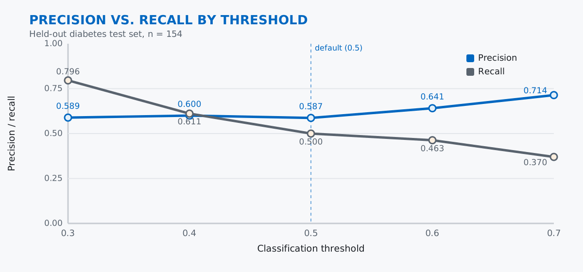

Lower the threshold to 0.3 and the model flags more patients as diabetic overall — recall climbs to 0.796 (it now catches about 80% of real diabetes cases) but precision drops slightly to 0.589, meaning more of those flags are false alarms. Raise it to 0.7 and the pattern reverses: precision climbs to 0.714 but recall collapses to 0.370, missing nearly two-thirds of the real cases. Neither end is objectively “better” — which one you’d actually pick depends on what a wrong answer costs in your specific situation, which is exactly the question the next section is about.

Four Gotchas Worth Knowing

0.5 is a convenient default, not a correct answer. A screening tool for a disease is a textbook case where the two mistakes aren’t equally costly: a false negative sends a diabetic patient home with no follow-up, while a false positive just costs an extra confirmatory test. That asymmetry argues for a lower threshold than 0.5 here, trading some precision for more recall — the 0.3 row above (0.796 recall) reads very differently once you think of it as “catches 80% of real cases” instead of “worse precision.” A fraud model guarding a high-friction manual review process might reasonably want the opposite. predict()’s built-in 0.5 is a default worth overriding deliberately, not a rule to follow silently.

Accuracy alone hides how a model handles the minority class. This model’s overall accuracy is 0.701. A model that predicted “no diabetes” for every single test patient — no learning at all — would score:

baseline_acc = (y_test == 0).mean()
model_acc = accuracy_score(y_test, y_pred)
baseline_acc, model_acc

(0.6493506493506493, 0.7012987012987013)

0.649 versus 0.701 — the fitted model only beats the do-nothing baseline by about 5 points of accuracy, even though its recall for the positive class is a real, useful 0.50. Accuracy compresses both classes into one number and lets the majority class dominate it; on an imbalanced target, always check the per-class precision and recall from the confusion matrix before trusting the headline accuracy figure.

Coefficients are on the log-odds scale — exponentiate before you say anything about probability. It’s tempting to see Pregnancies’ coefficient of 0.1157 and describe it as “each pregnancy adds about 11.6% to the probability of diabetes.” That’s wrong on two counts: it’s log-odds, not probability, and the odds ratio (e^0.1157 ≈ 1.1226) is a multiplier on the odds, not an addition to a percentage. “Each pregnancy multiplies the odds of a diabetes-positive prediction by about 1.12” is the version you can actually defend; anything that skips the exponentiation step is describing a number the model never produced.

A larger coefficient doesn’t mean a “more important” feature. This model deliberately used the eight features in their original, unscaled units instead of standardizing them first, which is exactly why max_iter had to go up — fitting on features with wildly different natural scales (Insulin in the hundreds, DiabetesPedigreeFunction under 3) is slower for the solver to converge on:

from sklearn.linear_model import LogisticRegression as LR
LR().fit(X_train, y_train)

/.../sklearn/linear_model/_logistic.py:599: ConvergenceWarning: lbfgs failed to converge after 100 iteration(s) (status=1):
STOP: TOTAL NO. OF ITERATIONS REACHED LIMIT

Increase the number of iterations to improve the convergence (max_iter=100).
You might also want to scale the data as shown in:
    https://scikit-learn.org/stable/modules/preprocessing.html
Please also refer to the documentation for alternative solver options:
    https://scikit-learn.org/stable/modules/linear_model.html#logistic-regression
  n_iter_i = _check_optimize_result(

Bumping max_iter to 1000 was the tradeoff made here on purpose: it keeps every coefficient in the feature’s own real-world units — “per mg/dL of glucose,” “per pregnancy” — instead of “per standard deviation,” which is harder to explain to a non-technical reader even though it would converge faster and make raw coefficient magnitudes more directly comparable. Neither choice is wrong; just be sure you know which one you made before comparing coefficient sizes across features.

Wrapping Up

One mental model, however many features: compute a linear combination of them (z), squash it through sigmoid into a probability, and threshold that probability into a class. Mapped onto the tools:

• z = w · x + b → the same linear combination LinearRegression stops at — logistic regression doesn’t
• sigmoid → turns any real number z into a probability between 0 and 1, unlike KNN, which never computes a z at all
• .predict_proba() → the probability underneath every .predict() label
• .coef_ → np.exp(.coef_) → log-odds weights turned into odds ratios you can actually explain
• confusion matrix / precision / recall → grade a classifier by more than one number, especially with an imbalanced target
• threshold → not fixed at 0.5; move it deliberately based on what a false positive costs versus a false negative

If you want the guided version of everything in this post — plus how to read an ROC curve and apply logistic regression to a new problem end to end — the introduction to logistic regression and interpreting the regression parameters lessons in our free Machine Learning course pick up exactly where this post leaves off.