An XGBoost regressor reports a mean absolute error of 4.88 seconds. Is that typical for this training workflow, or did one favorable data split make the model look better than it is? A single result cannot answer that question.

To measure XGBoost regression error with repeated cross-validation, reserve a final test set, run RepeatedKFold only on the remaining rows, and collect mean absolute error for every validation fold. Compare those fold errors with a simple baseline, inspect their mean and spread, then fit the unchanged model on all development rows and evaluate it once on the untouched test set.

This lesson predicts the runtime of fictional data exports. The workflow is designed for a beginner: first make the data boundaries clear, then evaluate one fixed set of model settings, and only then read the final test result.

Setup and files you need

You need Python 3.11 or newer and a terminal, script editor, or notebook. You should know that a regression model predicts a number, such as seconds, rather than a category. If fitting and predicting are new ideas, begin with How to Build Your First Machine Learning Model.

Create a virtual environment so this lesson’s packages do not change another project. On macOS or Linux, run these commands:

python -m venv .venv
source .venv/bin/activate
python -m pip install numpy pandas scikit-learn xgboost matplotlib

On Windows PowerShell, use .venv\Scripts\Activate.ps1 for the activation step. The executed build used Python 3.13.2, NumPy 2.5.1, pandas 3.0.3, scikit-learn 1.9.0, XGBoost 3.3.0, and Matplotlib 3.11.0.

Download data_export_runs.csv and save it beside your Python file. The dataset is original synthetic DataTweets data released under CC0-1.0. Synthetic means that code created the records. All 1,200 run IDs, export settings, and runtimes are fictional, so the results do not measure a real data platform.

Load the file and inspect only five rows. A small view makes the units and binary indicator columns easy to check:

import pandas as pd

exports = pd.read_csv("data_export_runs.csv")
print(exports.head(5).to_string(index=False))
print("shape:", exports.shape)

     run_id  source_rows  selected_columns  join_count  filter_selectivity_pct  concurrent_jobs  compressed_input  warm_cache  export_seconds
EXPORT-0001      1142976                37           1                    99.8                3                 1           0            55.7
EXPORT-0002      4109858                65           5                    11.8                2                 1           0           180.5
EXPORT-0003       525906                14           3                    92.8                5                 0           0            48.4
EXPORT-0004       134269                79           0                    14.6                1                 0           1            31.2
EXPORT-0005      5467519                62           4                    98.7                1                 0           1           177.9
shape: (1200, 9)

Each row is one completed export. The features are values known before the run finishes: row count, selected columns, joins, filter selectivity, concurrent jobs, compression, and cache state. The target is export_seconds, the number that the model learns to predict. In the compressed_input and warm_cache columns, 0 means no and 1 means yes.

Understanding what repeated cross-validation measures

A data split assigns rows to different jobs. Training rows teach the model. Validation rows measure a model choice during development. Test rows grade the completed workflow after those choices are fixed.

In five-fold cross-validation, the development data is divided into five parts called folds. The model trains on four folds and validates on the remaining fold. That process runs five times with a fresh fitted model each time, so every development row is used for validation once.

Repeated five-fold cross-validation creates new fold assignments and runs the five-fold process again. Three repetitions therefore fit 15 models and produce 15 validation errors. Each development row appears in a validation fold once per repetition:

960 development rows -> 5 folds x 3 repetitions -> 15 validation errors
240 test rows        -> kept closed until the workflow is fixed

The official scikit-learn RepeatedKFold reference defines it as repeated K-fold with different randomization in each repetition. A fixed random_state reproduces those assignments when the code runs again.

Why collect 15 errors instead of one? Their mean summarizes the model-fitting workflow across several partitions. Their minimum and maximum show how much the measured error changed. This spread is useful evidence about sensitivity to the split, but it is not a formal confidence interval. The fold results are related because the same rows appear in several training sets and in one validation fold per repetition.

Repeated random folds also assume that rows are independent and come from one stable process. They are wrong for time-ordered data when future rows must not train a model that predicts the past. They are also wrong when several rows belong to one customer, machine, or session. In those cases, use a time-aware or group-aware splitter.

Reserve the final test before evaluating folds

Name the seven feature columns explicitly. This keeps run_id and the answer column out of the model. Then reserve 20% of the rows for one final test:

from sklearn.model_selection import train_test_split

feature_columns = [
    "source_rows",
    "selected_columns",
    "join_count",
    "filter_selectivity_pct",
    "concurrent_jobs",
    "compressed_input",
    "warm_cache",
]

development, test = train_test_split(
    exports,
    test_size=0.20,
    random_state=20_260_722,
)

X_development = development[feature_columns]
y_development = development["export_seconds"]
X_test = test[feature_columns]
y_test = test["export_seconds"]

print(X_development.shape, X_test.shape)

(960, 7) (240, 7)

The 960 development rows will supply every training and validation fold. The 240 test rows must not influence the model settings, error metrics, or number of repetitions. Looking at their final score and then changing the workflow would turn the test set into another validation set.

Fix one XGBoost recipe and one baseline

XGBoost builds trees in sequence. Each new tree tries to correct error left by the trees before it. The current XGBRegressor API supplies a scikit-learn-compatible regression estimator, which means scikit-learn can clone and fit it inside every fold.

Define the model in a function. Cross-validation needs a fresh model for each split, and the function keeps the settings consistent between the repeated evaluation and the final fit:

from xgboost import XGBRegressor

def new_xgboost_model():
    return XGBRegressor(
        objective="reg:squarederror",
        tree_method="hist",
        n_estimators=260,
        learning_rate=0.045,
        max_depth=4,
        min_child_weight=5,
        subsample=0.9,
        colsample_bytree=0.9,
        reg_lambda=2.0,
        random_state=20_260_722,
        n_jobs=1,
    )

These settings are fixed teaching choices for this dataset, not recommended values for every problem. tree_method="hist" selects histogram tree building. n_jobs=1 also avoids competing levels of parallel work while scikit-learn controls the evaluation loop.

An error number needs context, so add DummyRegressor(strategy="median"). This baseline ignores all features and always predicts the median target from its current training fold. Because the median minimizes absolute error, it is a suitable simple baseline for MAE. The official DummyRegressor documentation describes dummy estimators as simple comparison rules, not useful final models.

Run 15 folds on the same partitions

Create the splitter and convert its output to a list. Reusing that list gives XGBoost and the baseline exactly the same training and validation indices:

from sklearn.model_selection import RepeatedKFold

repeated_folds = RepeatedKFold(
    n_splits=5,
    n_repeats=3,
    random_state=20_260_722,
)
fold_indices = list(repeated_folds.split(X_development, y_development))

print("validation scores per model:", len(fold_indices))
print("first fold rows:", len(fold_indices[0][0]), len(fold_indices[0][1]))

validation scores per model: 15
first fold rows: 768 192

Each validation fold has 192 rows, while its model trains on the other 768 development rows. The final test rows are not present in either count.

We will use two regression errors. Mean absolute error (MAE) is the average absolute difference between an actual value and its prediction. It stays in seconds, so an MAE of 5 means predictions are wrong by five seconds on average. Root mean squared error (RMSE) gives extra influence to larger errors, so it is usually at least as large as MAE.

cross_validate can collect both metrics and training scores. Scikit-learn follows a “higher is better” scorer convention, so loss names begin with neg_ and return negative values. Negate the returned arrays once to recover normal positive errors:

import numpy as np
from sklearn.dummy import DummyRegressor
from sklearn.model_selection import cross_validate

scoring = {
    "mae": "neg_mean_absolute_error",
    "rmse": "neg_root_mean_squared_error",
}

xgb_scores = cross_validate(
    new_xgboost_model(),
    X_development,
    y_development,
    cv=fold_indices,
    scoring=scoring,
    return_train_score=True,
    n_jobs=1,
)
baseline_scores = cross_validate(
    DummyRegressor(strategy="median"),
    X_development,
    y_development,
    cv=fold_indices,
    scoring=scoring,
    return_train_score=True,
    n_jobs=1,
)

xgb_validation_mae = -xgb_scores["test_mae"]
baseline_validation_mae = -baseline_scores["test_mae"]
print(np.round(xgb_validation_mae[:5], 2))

[4.88 4.81 5.35 5.01 4.67]

These are the XGBoost errors from the first repetition, not five metrics for one fitted model. Scikit-learn fitted a separate XGBoost model for every fold error. Its model-evaluation guide lists the negative scorer names and explains the sign convention.

Read the mean, spread, and train-validation gap

Build a compact table rather than reporting only the lowest fold. The sample standard deviation here describes the fold-to-fold spread of the 15 observed errors; it is not the uncertainty of the mean:

summary = pd.DataFrame({
    "method": ["XGBoost", "Median baseline"],
    "mean_cv_mae": [
        xgb_validation_mae.mean(),
        baseline_validation_mae.mean(),
    ],
    "std_cv_mae": [
        xgb_validation_mae.std(ddof=1),
        baseline_validation_mae.std(ddof=1),
    ],
    "minimum": [
        xgb_validation_mae.min(),
        baseline_validation_mae.min(),
    ],
    "maximum": [
        xgb_validation_mae.max(),
        baseline_validation_mae.max(),
    ],
})
print(summary.round(2).to_string(index=False))

         method  mean_cv_mae  std_cv_mae  minimum  maximum
        XGBoost         4.95        0.35     4.51     5.74
Median baseline        26.33        1.41    23.92    28.75

XGBoost’s mean validation MAE is 4.95 seconds, compared with 26.33 seconds for the median rule. Every observed XGBoost fold is also better than every baseline fold. That is stronger evidence than comparing two averages whose ranges overlap.

The XGBoost fold results move from 4.51 to 5.74 seconds. Report that variation instead of presenting 4.95 as an exact property of the model. A new sample from the same fictional process can still fall outside this observed range.

Training error provides one more diagnostic. Compare the mean training MAE with validation MAE and also read the average validation RMSE:

xgb_train_mae = -xgb_scores["train_mae"]
xgb_validation_rmse = -xgb_scores["test_rmse"]

print(f"mean training MAE:   {xgb_train_mae.mean():.2f} seconds")
print(f"mean validation MAE: {xgb_validation_mae.mean():.2f} seconds")
print(f"mean validation RMSE: {xgb_validation_rmse.mean():.2f} seconds")

mean training MAE:   2.60 seconds
mean validation MAE: 4.95 seconds
mean validation RMSE: 6.66 seconds

Training error is lower because each model is measured on rows it learned from. The 2.35-second gap shows that performance is more optimistic on those training rows. It can be a sign of overfitting, but the gap alone does not show whether the model is useful. RMSE is higher than MAE because larger misses receive more weight.

You can inspect every executed fold in repeated_cv_fold_metrics.csv. It includes repetition numbers, train MAE, validation MAE, validation RMSE, baseline errors, and fit time.

Open the test set once

The model recipe, splitter, metrics, and comparison rule are now fixed. Fit one fresh XGBoost model on all 960 development rows and evaluate its predictions on the 240 test rows:

from sklearn.metrics import mean_absolute_error, root_mean_squared_error

final_model = new_xgboost_model()
final_model.fit(X_development, y_development)
test_prediction = final_model.predict(X_test)

baseline = DummyRegressor(strategy="median")
baseline.fit(X_development, y_development)
baseline_prediction = baseline.predict(X_test)

print(
    f"XGBoost test MAE: "
    f"{mean_absolute_error(y_test, test_prediction):.2f} seconds"
)
print(
    f"XGBoost test RMSE: "
    f"{root_mean_squared_error(y_test, test_prediction):.2f} seconds"
)
print(
    f"Baseline test MAE: "
    f"{mean_absolute_error(y_test, baseline_prediction):.2f} seconds"
)

XGBoost test MAE: 4.32 seconds
XGBoost test RMSE: 5.70 seconds
Baseline test MAE: 26.08 seconds

The final MAE is below both the cross-validation mean and the observed 4.51-to-5.74-second fold range. That is possible for two reasons: the test set is another random sample, and the final model learned from all 960 development rows rather than the 768 rows available in each cross-validation fit. A fold range is not a promise about the test result. Do not rerun the split until the score moves closer to the cross-validation mean.

The generated chart combines the fold distribution with the final predictions:

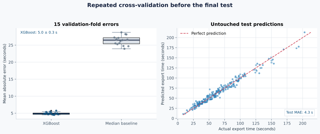
Read the left panel vertically: lower MAE is better, and each point is one validation fold. Read the right panel against the dashed diagonal. A point on that line is a perfect prediction; distance above or below it is the error for one export.

The executed test_predictions.csv lets you sort the final errors and inspect difficult rows. Do not use that inspection to tune the evaluated workflow and then report the same test score. Turn any new idea into a later experiment with new final test data.

Common mistakes and troubleshooting

You report the negative scorer values. neg_mean_absolute_error returns numbers such as -4.95 because scikit-learn ranks larger scores as better. Multiply by -1 once before calling the result MAE. Do not negate mean_absolute_error() itself; the metric function already returns a positive loss.

You run cross-validation on every row and then call the same rows a final test. Reserve test data first. Pass only the development features and target to cross_validate.

The baseline receives different folds. Materialize one split list and pass it to both evaluations. A paired comparison is easier to interpret because each method faces the same validation rows.

You choose the best fold as the result. The lowest error comes from a favorable partition; it is not an estimate of typical performance. Report all folds, their mean, and their spread. Keep unusual folds because they may reveal a real weakness.

You treat standard deviation as a confidence interval. Repeated folds share rows and are not independent experiments. Use the spread as a stability description. Formal uncertainty needs a statistical method whose assumptions match the data and evaluation design.

You tune settings during the same repeated evaluation and report its mean unchanged. Repeated cross-validation can compare fixed candidates, but choosing the winner adds model-selection bias. Use nested cross-validation or a separate tuning plan when you need an unbiased estimate after extensive search. The GridSearchCV accuracy-and-speed tutorial shows how to keep a final test outside selection.

Random folds ignore time or groups. Data-export runs from the same scheduled job may be more alike than independent runs. Keep related jobs together with group-aware validation. If production means predicting later runs from earlier runs, validate forward in time.

Your computer becomes slow during evaluation. Repeated five-fold validation fits 15 XGBoost models, plus 15 baselines in this lesson. Keep n_jobs=1 at both levels first. If you parallelize later, choose either the outer scikit-learn loop or XGBoost’s inner threads and watch memory use.

Your numbers differ slightly. Confirm the dataset, package versions, seed, column order, and model settings. CPU libraries can still introduce small numeric differences. Large differences usually indicate a changed split or feature list.

What you learned and what to test next

Repeated cross-validation changes the evaluation question from “What happened on one split?” to “How did the same model settings behave across several reasonable partitions?” For this synthetic export data, 15 XGBoost validation folds produced a mean MAE of 4.95 seconds, a standard deviation of 0.35 seconds, and a range from 4.51 to 5.74 seconds. The median baseline averaged 26.33 seconds.

The final XGBoost model reached an MAE of 4.32 seconds on 240 untouched rows. That result is consistent with the strong development results, but it remains evidence about one synthetic process and one fixed model recipe.

Carry four values into your next regression evaluation: the baseline error, the mean validation error, the fold spread, and the untouched test error. If the data has time, groups, or changing conditions, fix the splitter before tuning the model. A carefully chosen boundary is more valuable than another decimal place in the score.