Preparing Data for Machine Learning: Impute, Encode, and Scale in scikit-learn

Every “how to clean data” tutorial ends at a DataFrame with no missing values, and that DataFrame still isn’t something LogisticRegression().fit() will accept. Model classes want a matrix of numbers — no gaps, no strings — and a proper cleaning pass (our guide to cleaning messy data with pandas covers detecting and fixing that kind of mess) usually stops one step short of that. Turning categories like sex or embarked into numbers, filling the gaps a real dataset always has, and putting every feature on a comparable scale is a separate job, with a rule that’s easy to break without noticing: everything you learn about your data while doing this has to come only from the rows you’re allowed to train on.

The short version: split your data into training and test sets first. Then fit a SimpleImputer and StandardScaler on the numeric columns, and a separate SimpleImputer and OneHotEncoder on the categorical columns — but fit all of them using only the training rows. Bundle both column groups into one ColumnTransformer, chain that into a Pipeline with your model, and call .fit() once on the training data; the pipeline then applies the exact same, already-learned transformation to the test set with .transform(), so nothing about the test set ever shapes how the training data was prepared.

Why Fitting a Model Comes After Fitting Everything Else

An imputer’s fill value, a scaler’s mean and standard deviation, an encoder’s list of known categories — none of those are hardcoded. They’re all learned from data, the same way a model’s coefficients are learned from data. That’s the part people miss: a SimpleImputer computing “the mean age” and a LinearRegression computing “the coefficient on age” are doing the same kind of thing, just at different points in the pipeline.

Which means the leakage rule you already apply to the model — never let it see the test set during training — applies to every one of those preprocessing steps too. Compute a column’s mean, or catalog its categories, from the full dataset before you split, and a sliver of the test set’s information has already leaked into numbers your “training-only” model will use. The test score you get afterward is measuring something slightly more optimistic than what the model will actually do on truly new data.

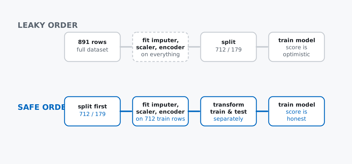
The fix is one rule, not a checklist: split first, fit second, and only ever fit on the training rows. Everything below is that rule applied to a real dataset with a real hole in it.

A Dataset With Real Holes to Patch

Titanic’s passenger manifest ships with seaborn, so there’s nothing to download — and it happens to have exactly the two problems this post is about: a numeric column with real gaps, and several columns that are plainly text.

import seaborn as sns

titanic = sns.load_dataset("titanic")
titanic.shape

(891, 15)

Data: the titanic dataset bundled with seaborn (public-domain historical passenger records from the 1912 sinking, digitized by the Encyclopedia Titanica project), loaded via sns.load_dataset("titanic").

titanic.isna().sum()

survived         0
pclass           0
sex              0
age            177
sibsp            0
parch            0
fare             0
embarked         2
class            0
who              0
adult_male       0
deck           688
embark_town      2
alive            0
alone            0
dtype: int64

deck is missing on 688 of 891 rows — over three-quarters of the column — so no imputation strategy makes it trustworthy; it’s dropped. class, embark_town, who, adult_male, and alone are all derived from or duplicate columns already in the table, and alive is just survived spelled differently, which would hand the model the answer for free. That leaves a compact, honest feature set:

features = ["pclass", "sex", "age", "sibsp", "parch", "fare", "embarked"]
target = "survived"
data = titanic[features + [target]].copy()
data.head()

   pclass     sex   age  sibsp  parch     fare embarked  survived
0       3    male  22.0      1      0   7.2500        S         0
1       1  female  38.0      1      0  71.2833        C         1
2       3  female  26.0      0      0   7.9250        S         1
3       1  female  35.0      1      0  53.1000        S         1
4       3    male  35.0      0      0   8.0500        S         0

Ticket class, sex, age, family size, fare, and where each passenger boarded — a mix of numbers and text, with age and embarked still carrying the gaps from the table above. (Outputs in this post are from pandas 3.0.3 and scikit-learn 1.9.0.)

What Happens If You Skip Straight to .fit()

It’s worth seeing the actual failure once, because the error message is the whole motivation for this post:

from sklearn.linear_model import LogisticRegression

X = data[features]
y = data[target]

LogisticRegression().fit(X, y)

ValueError: could not convert string to float: 'male'

scikit-learn’s estimators expect a purely numeric array underneath the DataFrame. The moment it hits the sex column, it has no idea what to do with the string "male" — and it would have failed just as fast on the NaN values in age if sex weren’t first in line. Both problems need solving before any model gets near this data.

Split First, Then Everything Else Follows From the Training Set

Reach for train_test_split before you touch an imputer or scaler, not after:

from sklearn.model_selection import train_test_split

X_train, X_test, y_train, y_test = train_test_split(
    X, y, test_size=0.2, random_state=42, stratify=y
)
X_train.shape, X_test.shape

((712, 7), (179, 7))

stratify=y keeps the survival rate roughly equal between the two sets, which matters here because more passengers died than survived. Now watch what “fit on everything” versus “fit on training only” actually costs you, using something as simple as the mean of age:

full_mean_age = X["age"].mean()
train_mean_age = X_train["age"].mean()
print(f"mean age, full dataset:  {full_mean_age:.4f}")
print(f"mean age, training only: {train_mean_age:.4f}")

mean age, full dataset:  29.6991
mean age, training only: 29.8077

Two different numbers, from two different populations. If an imputer fit on the full dataset fills every gap with 29.6991, some of those fills are informed — however slightly — by rows the model is never supposed to have seen yet. Fit on X_train alone and every downstream number is honestly training-only, which is the entire point of having a test set in the first place.

Two Preprocessing Pipelines, One Per Column Type

Numeric and categorical columns need different treatment, so build each as its own small Pipeline. For the numeric columns — pclass, age, sibsp, parch, fare — fill gaps with the median, then scale:

from sklearn.impute import SimpleImputer
from sklearn.pipeline import Pipeline
from sklearn.preprocessing import StandardScaler

numeric_cols = ["pclass", "age", "sibsp", "parch", "fare"]

numeric_pipeline = Pipeline([
    ("impute", SimpleImputer(strategy="median")),
    ("scale", StandardScaler()),
])

For the categorical columns — sex and embarked — fill gaps with the most frequent value, then one-hot encode:

from sklearn.preprocessing import OneHotEncoder

categorical_cols = ["sex", "embarked"]

categorical_pipeline = Pipeline([
    ("impute", SimpleImputer(strategy="most_frequent")),
    ("encode", OneHotEncoder(handle_unknown="ignore")),
])

Neither of these does anything yet — a Pipeline object, like the DataFrameGroupBy object pandas hands back from .groupby(), is a plan, not a result. It waits for .fit() or .fit_transform() before it learns a single number.

Combining Both With ColumnTransformer

A ColumnTransformer routes each pipeline to its own columns and stitches the results back into one array. This is where “fit only on training data” becomes a single line rather than something you have to remember to do twice:

from sklearn.compose import ColumnTransformer

preprocessor = ColumnTransformer([
    ("num", numeric_pipeline, numeric_cols),
    ("cat", categorical_pipeline, categorical_cols),
])

X_train_transformed = preprocessor.fit_transform(X_train)
X_test_transformed = preprocessor.transform(X_test)

print("X_train raw:", X_train.shape, "-> transformed:", X_train_transformed.shape)
print("X_test raw: ", X_test.shape, "-> transformed:", X_test_transformed.shape)

X_train raw: (712, 7) -> transformed: (712, 10)
X_test raw:  (179, 7) -> transformed: (179, 10)

Note the asymmetry that’s easy to miss: fit_transform on the training set, but plain transform on the test set. Seven columns became ten because sex and embarked each exploded into one column per category. You can see exactly which ones:

preprocessor.get_feature_names_out()

array(['num__pclass', 'num__age', 'num__sibsp', 'num__parch', 'num__fare',
       'cat__sex_female', 'cat__sex_male', 'cat__embarked_C',
       'cat__embarked_Q', 'cat__embarked_S'], dtype=object)

sex (2 categories) plus embarked (3 categories) accounts for the extra 5 columns on top of the original 5 numeric ones. This is exactly the moment where a high-cardinality column — a city field with 200 distinct values, say — would quietly balloon your feature count; that’s a real cost of one-hot encoding worth remembering, even though it isn’t a problem for a 2- and 3-category column like these. The full scikit-learn Pipeline and ColumnTransformer guide covers routing columns by dtype, nesting transformers, and more than this post needs.

Chaining Preprocessing and the Model Together

Wrap the ColumnTransformer and a classifier into one final Pipeline, and .fit() does both jobs in the right order with a single call:

clf = Pipeline([
    ("preprocess", preprocessor),
    ("model", LogisticRegression(max_iter=1000)),
])

clf.fit(X_train, y_train)
predictions = clf.predict(X_test)

from sklearn.metrics import accuracy_score
round(accuracy_score(y_test, predictions), 4)

0.8045

80.45% of the held-out passengers were classified correctly, and — because the whole preprocessing chain lives inside the same Pipeline object as the model — that number reflects a model that never saw a single test-set value while deciding how to fill gaps, scale numbers, or list categories. Call clf.predict() on brand-new data later and the same fitted imputer, scaler, and encoder run automatically; there’s no second script to keep in sync with the training one.

Two Ways This Still Bites You

A category in the test set that the training set never saw. Real data drifts — a shipping route with a port that never showed up in your training window, a product category added last month. Force the point with a training slice that happens to contain only one embarked value:

train_small = X_train.iloc[:50].copy()
train_small["embarked"] = "S"

strict_encoder = OneHotEncoder(handle_unknown="error")
strict_encoder.fit(train_small[["embarked"]])
strict_encoder.transform(X_test[["embarked"]])

ValueError: Found unknown categories ['C', 'Q'] in column 0 during transform

handle_unknown="error" is the strict default, and it just refused to transform data with categories it never learned. Switch it to "ignore" and unseen categories get encoded as all zeros instead of raising:

safe_encoder = OneHotEncoder(handle_unknown="ignore")
safe_encoder.fit(train_small[["embarked"]])
safe_encoder.transform(X_test[["embarked"]].iloc[:3]).toarray()

array([[1.],
       [1.],
       [0.]])

Those three test rows are actually S, S, C — the encoder only ever learned S, so it correctly flags the two S rows and quietly zeroes out the C row instead of crashing the whole prediction. That’s the entire reason the pipeline earlier used handle_unknown="ignore" rather than the stricter default.

Mean imputation on a skewed column. fare isn’t close to symmetric — a handful of first-class tickets stretch the top of the distribution far past everyone else:

print(f"fare mean:   {X_train['fare'].mean():.2f}")
print(f"fare median: {X_train['fare'].median():.2f}")
print(f"fare max:    {X_train['fare'].max():.2f}")

fare mean:   31.82
fare median: 14.45
fare max:    512.33

A single fare of 512 pulls the mean more than twice as high as the median. Impute missing fares with the mean and you’d be filling gaps with a number more than half the passengers never paid anywhere close to; the median is the more honest stand-in for a typical passenger, which is why the numeric pipeline above used strategy="median" rather than the default "mean". As a quick gut check: does a column’s mean sit noticeably far from its median? If so, median imputation is usually the safer default.

None of this machinery is universal, either — tree-based models like XGBoost can split directly on missing values and raw categorical columns without an imputer or encoder at all, which our post on handling missing values in XGBoost without imputation walks through on its own dataset. Linear models and anything scale-sensitive, like the logistic regression here, don’t get that shortcut.

Every column that reaches .fit() now carries only what the training rows taught it, in the order split, then fit, then transform. That’s the same discipline the machine learning workflow lesson in our free Machine Learning course builds a full classifier around — and if your last stop was training a model on data that was already numeric and complete, our post on training your first machine learning model is the fit-predict-evaluate half of the story this one was missing.