Monitor LLM Requests with JSONL and pandas in Python

An LLM application can keep returning answers while becoming slower, less reliable, or more expensive to run. A successful manual test will not reveal a timeout that affects one request in twenty. It will also not show whether a prompt update adds hundreds of input tokens to every call.

This tutorial builds a small monitoring report for a fictional information assistant. We will compare a baseline release with a candidate release using saved request records. The report measures successful requests, median and 95th-percentile latency, and total token use. It then applies three clear checks before the candidate can move forward.

The lesson does not call a model service. Its 240 records are original synthetic teaching data, so the same code produces the same result on every run. The numbers do not describe a real provider or model. They let us learn the monitoring method without an API key, private user text, or a changing bill.

Prerequisites and Setup

You need Python 3.10 or later. You should know how to run a Python file, but you do not need monitoring experience. A pandas DataFrame is a table with named columns. We use pandas to summarize the request records and Matplotlib to create the comparison chart.

Create a virtual environment, activate it, and install both packages. On macOS or Linux, run:

python -m venv .venv
source .venv/bin/activate
python -m pip install pandas matplotlib

On Windows PowerShell, use .venv\Scripts\Activate.ps1 for the activation command.

The executed build used Python 3.13.2, pandas 3.0.3, and Matplotlib 3.11.0. Download the synthetic LLM request traces and save the file beside your Python script.

The dataset was generated deterministically for this lesson and is released under CC0 1.0. All request IDs, timestamps, versions, request types, statuses, token counts, and durations are fictional. No prompt, answer, name, account number, or other user content is present.

Mental Model: One Request Becomes One Record

Observability means collecting enough evidence to understand what a running system did. For this lesson, each completed model request becomes one trace record. A trace is a structured account of one operation. It answers a few focused questions:

• Which release and prompt version received the request?
• What kind of work was requested?
• Did the operation succeed?
• How many input and output tokens did it use?
• How long did it take from start to finish?

The first dataset row looks like this:

{"request_id":"REQ-1-001","started_at_utc":"2026-06-01T08:00:00Z","release":"baseline","prompt_version":"faq-v1","request_type":"opening_hours","status":"ok","input_tokens":247,"output_tokens":68,"latency_ms":623}

The file uses JSON Lines, often shortened to JSONL. Each line is one complete JSON object. That layout is useful for event data because a program can append a new record without rewriting one large JSON array. pandas reads this format when read_json() receives lines=True, as shown in its current read_json documentation.

If JSONL is new to you, the DataTweets tutorial on processing large JSON files with pandas explains how the format can also be read in chunks.

This schema is intentionally smaller than a full tracing standard. The current OpenTelemetry generative AI metric conventions include operation duration and input/output token use. Those conventions are still marked as development, so check their status before adopting exact names in a long-lived system. The durable idea is to give each measurement a clear meaning and unit.

Notice what the schema omits. Raw prompts and answers may contain personal or confidential information. Start with operational fields. Add content only when there is a reviewed need, a retention policy, and suitable access control.

Load and Validate the Traces

Load one JSON object per line and ask pandas to parse the UTC timestamp. convert_dates names the column that should become a datetime value rather than plain text.

from pathlib import Path

import pandas as pd

trace_path = Path("llm_request_traces.jsonl")
traces = pd.read_json(
    trace_path,
    lines=True,
    convert_dates=["started_at_utc"],
)

Do not calculate metrics before checking the table. A duplicate request can be counted twice. A negative duration has no useful meaning here. An unexpected status could be silently treated as a failure, hiding an upstream schema change.

The next checks make those assumptions executable:

required_columns = {
    "request_id", "started_at_utc", "release", "prompt_version",
    "request_type", "status", "input_tokens", "output_tokens",
    "latency_ms",
}

assert required_columns.issubset(traces.columns)
assert traces["request_id"].is_unique
assert traces["started_at_utc"].dt.tz is not None
assert (traces[["input_tokens", "output_tokens", "latency_ms"]] >= 0).all().all()
assert set(traces["status"]) == {"ok", "timeout", "provider_error"}

print(f"rows={len(traces)} unique_ids={traces['request_id'].nunique()}")
print("releases:", sorted(traces["release"].unique()))
print("statuses:", sorted(traces["status"].unique()))

The generated file passed every assertion and printed:

rows=240 unique_ids=240
releases: ['baseline', 'candidate']
statuses: ['ok', 'provider_error', 'timeout']

There are 240 rows and 240 IDs, so no request is duplicated. The two release names are available for comparison. The status list also matches the policy used by this lesson.

An assertion stops the script when an assumption is false, unless Python is run with assertions disabled. In a scheduled data pipeline, replace bare assertions with validation that records the reason and exits with a non-zero status. The core rule stays the same: reject an unclear monitoring table instead of publishing a confident but wrong report.

Calculate Reliability, Latency, and Token Use

We need two derived columns. successful is True only for an ok row. Because Python treats True as 1 and False as 0 in this calculation, its group mean is the success rate. total_tokens adds the input and output counts reported for a request.

traces["successful"] = traces["status"].eq("ok")
traces["total_tokens"] = (
    traces["input_tokens"] + traces["output_tokens"]
)

Now group by release. A percentile is a position in an ordered set of values. The 50th percentile, or median, describes a typical request. The 95th percentile is the value at or below which about 95% of observations fall. It helps expose the slow end of the distribution that an average can hide.

summary = (
    traces.groupby("release", sort=False)
    .agg(
        requests=("request_id", "size"),
        success_rate=("successful", "mean"),
        p50_latency_ms=("latency_ms", "median"),
        p95_latency_ms=(
            "latency_ms",
            lambda values: values.quantile(0.95),
        ),
        mean_total_tokens=("total_tokens", "mean"),
    )
    .reset_index()
)

for column in ("p50_latency_ms", "p95_latency_ms", "mean_total_tokens"):
    summary[column] = summary[column].round().astype(int)

print(summary.to_string(index=False))

pandas defines quantile(0.95) as the 95th-percentile calculation. Its grouped quantile reference also documents how values between observed points are interpolated.

The executed summary was:

  release  requests  success_rate  p50_latency_ms  p95_latency_ms  mean_total_tokens
 baseline       120      0.983333             983            1250                404
candidate       120      0.941667            1728            2032                664

Read the rows from left to right. The baseline completed 98.3% of requests successfully. Its typical latency was 983 milliseconds, while its slower tail reached 1,250 milliseconds. The candidate had a 94.2% success rate, a median latency of 1,728 milliseconds, and mean usage of 664 tokens per request.

This report includes failed operations in the latency and token calculations. That choice reflects the resources and waiting time users experienced. Another team may report successful and failed requests separately. Either policy can work, but it must stay consistent across releases.

Token count is a usage measure, not a price. A provider may use different token rules or billing categories. Prefer the usage returned by the model service. Do not convert tokens to money until you have current prices and know which token types are billable.

Turn the Summary into a Release Gate

A chart helps people inspect a change, but an automated process needs a decision. A release gate is a set of checks that must pass before software moves to the next stage.

Choose limits before reading the candidate result. Otherwise, it is easy to adjust a limit only to make a preferred release pass. These are teaching limits for the fictional assistant, not universal targets:

limits = {
    "minimum_success_rate": 0.95,
    "maximum_p95_latency_ms": 1750,
    "maximum_mean_total_tokens": 650,
}

The check function compares one summary row with all three limits. all() returns True only when every check passes.

def check_release(row):
    checks = {
        "success_rate": (
            row["success_rate"] >= limits["minimum_success_rate"]
        ),
        "p95_latency_ms": (
            row["p95_latency_ms"] <= limits["maximum_p95_latency_ms"]
        ),
        "mean_total_tokens": (
            row["mean_total_tokens"]
            <= limits["maximum_mean_total_tokens"]
        ),
    }
    return checks, all(checks.values())

for _, row in summary.iterrows():
    checks, passed = check_release(row)
    failed = [name for name, result in checks.items() if not result]
    decision = "PASS" if passed else "BLOCK"
    detail = "none" if not failed else ", ".join(failed)
    print(f"{row['release']} gate={decision} failed_checks={detail}")

The executed gate output was:

baseline gate=PASS failed_checks=none
candidate gate=BLOCK failed_checks=success_rate, p95_latency_ms, mean_total_tokens

The candidate misses the minimum success rate by about 0.8 percentage points. Its p95 latency is 282 milliseconds above the limit, and its mean token use is 14 tokens above the budget. The correct automated decision is BLOCK.

Blocking is not the same as deleting the change. It creates a clear next action: inspect why the candidate changed, improve it, then generate a fresh set of comparable traces. A team could also require human approval for an accepted exception, but the exception should be recorded rather than hidden by editing the result.

Find the Request Type Behind the Slow Tail

One release-level row tells us that a problem exists. It does not tell us where to start. Break the candidate down by request_type while keeping the same definitions for latency and tokens.

candidate_by_type = (
    traces.loc[traces["release"].eq("candidate")]
    .groupby("request_type", sort=False)
    .agg(
        requests=("request_id", "size"),
        p95_latency_ms=(
            "latency_ms",
            lambda values: round(values.quantile(0.95)),
        ),
        mean_total_tokens=("total_tokens", lambda values: round(values.mean())),
    )
    .reset_index()
)

print(candidate_by_type.to_string(index=False))

The executed breakdown was:

        request_type  requests  p95_latency_ms  mean_total_tokens
        opening_hours        40            1636                569
    document_checklist        40            1887                668
     application_status        40            2108                756

application_status is the first category to inspect. It has the highest tail latency and token use. opening_hours stays within both displayed maximums. That difference suggests checking category-specific context instead of shortening every response without evidence.

Forty synthetic observations per category are enough to show the method, but not enough to define a production target. Tail percentiles can change sharply when the sample is small. Use a time window and request volume that represent your traffic, and show the number of observations beside every percentile.

Read the Generated Monitoring Chart

The build script turns the summary into three side-by-side checks. Each dashed line is the limit used by the release gate.

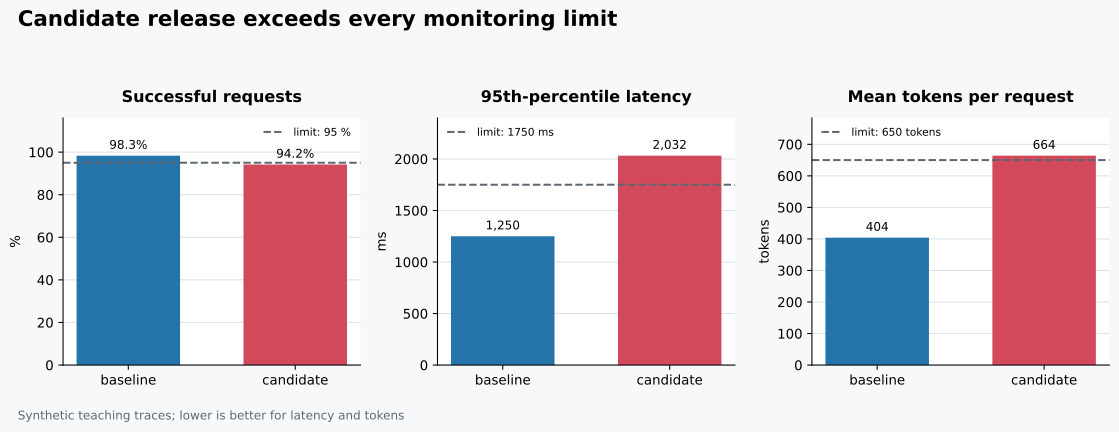
The left panel is different from the other two: a higher success rate is better. For latency and token use, lower bars are better. The candidate bar falls below the success line and rises above both maximum lines. The picture and gate therefore tell the same story.

Keep the numeric table with the chart. A chart helps readers see the direction and size of change, while the table gives the exact values needed for a check or incident note.

Common Mistakes and Troubleshooting

read_json() raises a trailing-data error. Confirm that the file contains one object per line and pass lines=True. A JSON array surrounded by [ and ] is a different layout.

The timestamp column has no .dt accessor. pandas did not parse it as a datetime. Pass the column through convert_dates, then check that each input timestamp includes a time-zone offset or Z for UTC.

Only mean latency is reported. An average can look acceptable while a small group waits much longer. Include a tail measure such as p95 and always show its sample count.

Failed requests disappear before aggregation. Filtering to status == "ok" can make reliability and latency look better than the user experience. Count every request for the success rate. State clearly whether latency and usage include failures.

Prompt text and answers are logged by default. These fields can contain secrets or personal data. Collect the least data needed, remove credentials, limit access, and set a retention period. A request ID can connect an operational record to protected detail stored elsewhere.

Several changes share one release label. If a prompt, model, retrieval index, and runtime change together, the report cannot identify which change caused the regression. Record the versions that matter and change one part at a time when possible.

Token counts are estimated from character length. Character-based estimates vary across tokenizers and languages. Use provider-reported input and output usage when it is available. If it is unavailable, mark an estimate as an estimate instead of mixing it with measured counts.

The synthetic result is treated as a benchmark. This dataset teaches calculations only. It does not support a claim about a real model’s speed, reliability, quality, or cost. Build a separate governed trace dataset from your own system before making an operational decision.

Recap

Useful monitoring starts with a small, explicit record for each request:

• identify the release, prompt version, request type, and status;
• store duration and provider-reported input and output token counts;
• validate IDs, time zones, statuses, and non-negative measurements;
• compare success rate, typical latency, tail latency, and token use;
• apply limits chosen before the candidate result is known; and
• break a failed release into meaningful categories before changing it.

The durable mental model is record, validate, summarize, decide, diagnose. A full tracing platform can automate collection and storage later. The small pandas report remains valuable because its definitions and release decision are visible, testable, and easy to reproduce.