Netflix Viewing History: Parsing, Deriving, and Summarizing Your Data

“How much of my free time actually went to three shows?” is a question you can only answer with your own data, and Netflix will hand it to you: every account lets you download a full viewing history as a plain CSV. Most people download it, open it once, and close it again, because the file is just two columns of raw text and doesn’t answer anything by itself.

That’s where this project picks up. The export is a flat, one-row-per-episode log with dates in a format that’s easy to misread, and turning it into real answers — your most-watched shows, your busiest viewing day, your actual weekday habits — takes a few deliberate pandas moves. If you haven’t worked with Python’s date tools before, our Python datetime guide covers the fundamentals this project leans on. Below, we build the mental model first, then work through it hands-on on a sample file shaped exactly like your real export.

The Mental Model: Parse, Derive, Summarize

Every question you’ll ask of a viewing history — “which day do I watch the most?”, “what was my biggest binge?” — routes through the same three moves, in the same order:

1. Parse the raw date text into real datetime values pandas can do arithmetic on.
2. Derive new columns from what you parsed — the day of the week, the month, whether a row was a weekend — and from the title text itself, like pulling a show’s name out of its episode title.
3. Summarize with a count or a groupby to collapse hundreds of rows into the handful of numbers you actually came for.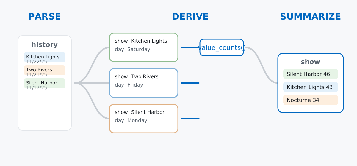

You’ll reach for parse once per column, derive a handful of times, and summarize differently for every question — but the shape never changes.

A Dataset You Can Reproduce (Shaped Like Netflix’s Own Export)

Netflix’s export (Account → Profile and Parental Controls → Download your personal information → Viewing activity) is a CSV with exactly two columns: Title and Date. There’s one row per thing you pressed play on — an episode, a movie, even a trailer — with the episode’s season and number folded into the Title string and the date written as US-style M/D/YY text.

That file is inherently personal, so there’s nothing to vendor here. Instead, generate a sample file with the same two columns and the same quirks, seeded so your numbers match this post exactly. Imagine a year of watching two Netflix originals with a mix of movie nights on the side:

import numpy as np
import pandas as pd

rng = np.random.default_rng(42)

shows = {
    "Silent Harbor": 8,
    "Kitchen Lights": 10,
    "Nocturne": 6,
    "Paper Cities": 9,
}
movies = ["Midnight Ferry", "Two Rivers", "The Understudy", "Low Tide"]

all_days = pd.date_range("2025-01-01", periods=334, freq="D")
weekend_boost = np.where(all_days.dayofweek >= 4, 3, 1)
day_weights = weekend_boost / weekend_boost.sum()

rows = []
for _ in range(90):
    day = rng.choice(all_days, p=day_weights)
    if rng.random() < 0.65:
        show = rng.choice(list(shows))
        total_eps = shows[show]
        count = min(int(rng.integers(1, 5)), total_eps)
        start_ep = int(rng.integers(1, total_eps - count + 2))
        for ep in range(start_ep, start_ep + count):
            rows.append((f"{show}: Season 1: Episode {ep}", day))
    else:
        movie = rng.choice(movies)
        rows.append((movie, day))

history = pd.DataFrame(rows, columns=["Title", "Date"])
history = history.sort_values("Date", ascending=False).reset_index(drop=True)
history["Date"] = history["Date"].dt.strftime("%m/%d/%y")
history.to_csv("netflix_viewing_history.csv", index=False)

history.head()

                                  Title      Date
0                        Midnight Ferry  11/29/25
1  Kitchen Lights: Season 1: Episode 10  11/22/25
2                            Two Rivers  11/22/25
3                            Two Rivers  11/21/25
4    Silent Harbor: Season 1: Episode 7  11/17/25

185 rows, exactly two columns, dates as plain text — that’s the real shape of a Netflix export, weekend-heavy rng.choice weighting and all. (The outputs in this post come from pandas 3.0; everything shown also works on pandas 2.x.) Once you have your own NetflixViewingHistory.csv, every line below works unchanged — just swap the filename in the next step.

Loading and Parsing the Dates

Read the file back the way you’d read your own download, then check what pandas actually gave you:

history = pd.read_csv("netflix_viewing_history.csv")
history.dtypes

Title    str
Date     str
dtype: object

Both columns come in as text. (Pandas 3.0 labels string columns str here — on pandas 2.x the same columns show as object; either way, Date isn’t a real date yet.) Convert it explicitly, naming the format instead of letting pandas guess:

history["Date"] = pd.to_datetime(history["Date"], format="%m/%d/%y")
history.dtypes

Title               str
Date     datetime64[us]
dtype: object

Date is now datetime64, which means you can sort it, subtract it, and pull calendar fields out of it — none of which work on plain text.

Deriving Calendar Features

With a real datetime column, .dt unlocks calendar-level questions with no manual parsing:

history["day_of_week"] = history["Date"].dt.day_name()
history["month"] = history["Date"].dt.month_name()
history["is_weekend"] = history["Date"].dt.dayofweek >= 4

history[["Title", "Date", "day_of_week", "is_weekend"]].head()

                                  Title       Date day_of_week  is_weekend
0                        Midnight Ferry 2025-11-29    Saturday        True
1  Kitchen Lights: Season 1: Episode 10 2025-11-22    Saturday        True
2                            Two Rivers 2025-11-22    Saturday        True
3                            Two Rivers 2025-11-21      Friday        True
4    Silent Harbor: Season 1: Episode 7 2025-11-17      Monday       False

day_of_week and is_weekend are new columns computed straight from Date — nothing here required looking at the calendar by hand or writing a lookup table.

Which Day of the Week You Actually Watch

Group by the derived day_of_week column and count rows per group, reindexing to Monday-through-Sunday order since groupby sorts alphabetically by default:

weekday_order = ["Monday", "Tuesday", "Wednesday", "Thursday", "Friday", "Saturday", "Sunday"]
history.groupby("day_of_week").size().reindex(weekday_order)

day_of_week
Monday       23
Tuesday       3
Wednesday    15
Thursday     13
Friday       32
Saturday     56
Sunday       43
dtype: int64

Saturday is the clear peak here, with Tuesday barely registering — a pattern that’s easy to describe in words but only became a number once the date was parsed and the weekday derived from it.

Extracting the Show Name from Episode Titles

Netflix folds the season and episode into Title, so "Kitchen Lights: Season 1: Episode 10" and the movie "Two Rivers" need to become one comparable show column. A str accessor split on the first colon does it for both cases at once:

history["show"] = history["Title"].str.split(":").str[0]
history[["Title", "show"]].head()

                                  Title            show
0                        Midnight Ferry  Midnight Ferry
1  Kitchen Lights: Season 1: Episode 10  Kitchen Lights
2                            Two Rivers      Two Rivers
3                            Two Rivers      Two Rivers
4    Silent Harbor: Season 1: Episode 7   Silent Harbor

str.split(":") turns each title into a list of pieces, and .str[0] grabs the first one — the show or movie name, whether or not a season/episode suffix followed it. Pandas’ string-handling user guide covers the rest of the str accessor if you want to go further than a single split.

Your Most-Watched Titles

With one consistent show column, value_counts answers the question the whole project started with:

history["show"].value_counts().head(6)

show
Silent Harbor     46
Kitchen Lights    43
Nocturne          34
Paper Cities      31
The Understudy    10
Midnight Ferry     8
Name: count, dtype: int64

Each show’s count is a row count, not an episode count — every play, including the odd rewatched episode, is counted once. Silent Harbor narrowly edges out Kitchen Lights for the top spot, and the four movies trail every series by a wide margin.

Finding Your Biggest Binge Day

Group by the parsed Date this time instead of a derived column, and the day with the most rows is, by definition, the day you watched the most in one sitting:

daily_counts = history.groupby("Date").size().sort_values(ascending=False)
daily_counts.head()

Date
2025-10-04    9
2025-07-05    8
2025-09-19    5
2025-03-08    5
2025-01-06    4
dtype: int64

Pull the top day’s index value back out and filter the original table with it to see exactly what made up that binge:

top_day = daily_counts.index[0]
history.loc[history["Date"] == top_day, ["Title"]]

                                 Title
26  Silent Harbor: Season 1: Episode 3
27  Silent Harbor: Season 1: Episode 4
28  Silent Harbor: Season 1: Episode 5
29  Silent Harbor: Season 1: Episode 1
30  Silent Harbor: Season 1: Episode 4
31  Silent Harbor: Season 1: Episode 6
32  Silent Harbor: Season 1: Episode 7
33                      Midnight Ferry
34  Silent Harbor: Season 1: Episode 2

Nine plays on one day, mostly Silent Harbor out of order — including episode 4 twice, which is exactly the kind of messy, human detail a real viewing history has and a clean synthetic one usually wouldn’t bother including.

Three Gotchas Worth Knowing

Skipping format= leaves the date reading up to a guess, and the guess can be wrong for you specifically. Two-digit day/month pairs like 3/4/25 are genuinely ambiguous — is that March 4th or April 3rd? Netflix’s export is always month-first, but a reader used to day-first dates who reaches for dayfirst=True gets a silently different answer:

sample = pd.Series(["3/4/25", "12/1/25"])
pd.to_datetime(sample, dayfirst=True)

0   2025-04-03
1   2025-01-12
dtype: datetime64[us]

pd.to_datetime(sample, format="%m/%d/%y")

0   2025-03-04
1   2025-12-01
dtype: datetime64[us]

Both calls run without error and return two clean dates — they just disagree with each other on every row. Naming the format explicitly is the only way to be sure which one you got; pandas will also warn you in the console (“Could not infer format…”) whenever you skip it.

Splitting on : breaks the moment a title has its own colon. The str.split(":").str[0] trick from earlier assumes the first colon always separates the name from the season/episode suffix — which fails for a movie subtitle:

edge_case = pd.Series(["Low Tide: Anniversary Edition", "Silent Harbor: Season 1: Episode 4"])
edge_case.str.split(":").str[0]

0         Low Tide
1    Silent Harbor
dtype: object

"Low Tide: Anniversary Edition" gets truncated to just "Low Tide", silently dropping “Anniversary Edition” — fine if you only care about the base title, a real bug if you don’t. Check a sample of your own show column against the original Title before trusting it.

A formatted date string still sorts as text unless you convert it back. After .dt.strftime(), Date looks like a date but behaves like any other string — sort_values() on it goes alphabetically, not chronologically:

messy = pd.Series(["9/1/25", "10/1/25", "2/1/25"])
messy.sort_values().tolist()

['10/1/25', '2/1/25', '9/1/25']

October lands before February because "1" sorts before "2" as a character. Parse first, sort second:

pd.to_datetime(messy, format="%m/%d/%y").sort_values().dt.strftime("%m/%d/%y").tolist()

['02/01/25', '09/01/25', '10/01/25']

Wrapping Up

Every question in this project came down to the same three moves:

• Parse — pd.to_datetime(..., format=...) turns export text into real dates, on your terms instead of a guess.
• Derive — .dt.day_name(), .dt.dayofweek, and str.split(":").str[0] pull calendar and title features out of what you parsed.
• Summarize — value_counts() and groupby(...).size() collapse the parsed, derived table into the actual answers you wanted.

The same three moves apply directly to your own download — just point pd.read_csv at your real NetflixViewingHistory.csv and rerun everything from the parsing step on. If you want the fuller course version of this workflow — date arithmetic, filtering by date ranges, and time-based grouping with more exercises — the DateTime Fundamentals lesson in our free Python for Data Analytics course picks up exactly where this post’s parsing section leaves off.