Neural Network Classification in Python with Scikit-Learn

A sensor table can contain patterns that a straight decision boundary misses. High motor temperature may be safe when vibration is low, while the same temperature may signal a problem when vibration is high. These interactions are one reason to try a small neural network on tabular data.

This tutorial builds a binary classifier that predicts whether a fictional conveyor will fail its next inspection. Binary classification means choosing between two labels: pass (0) or fail (1). We will use a multilayer perceptron, or MLP, from scikit-learn. An MLP is a feed-forward neural network made from connected layers of small calculation units called neurons.

This is a focused first neural-network project. It does not need a graphics processor, cloud account, or image dataset. You will see each important step, the real output from an executed script, and the mistakes that often make a first model look better than it is. If supervised learning is new to you, read How to Build Your First Machine Learning Model first for the general train-and-test workflow.

What You Need Before You Begin

You need Python 3.11 or newer and basic familiarity with variables, functions, and pandas DataFrames. A DataFrame is pandas’ table structure: rows hold observations and columns hold variables. Create a virtual environment if you want to keep this project’s packages separate from other projects, then install the four packages used here:

python -m venv .venv
source .venv/bin/activate
python -m pip install numpy pandas scikit-learn matplotlib

The results shown below were produced with Python 3.13.2, pandas 3.0.3, scikit-learn 1.9.0, NumPy 2.5.1, and Matplotlib 3.11.0. Small numerical differences can occur with other package versions or computer systems.

The complete dataset is available as conveyor_sensor_readings.csv. It is an original synthetic dataset generated with NumPy and random seed 27. “Synthetic” means the rows were produced by code rather than collected from real equipment. All measurements and labels are fictional, so this model must not be used for real safety decisions. The dataset is released under CC0 1.0, which permits reuse without restriction.

Load the CSV and inspect a small sample before building a model. This confirms the column names and makes the target format visible.

import pandas as pd

sensor_data = pd.read_csv(
    "https://datatweets.com/datasets/blog/"
    "neural-network-classification-python/conveyor_sensor_readings.csv"
)

print(sensor_data.shape)
print(sensor_data.head(3).to_string(index=False))
print(sensor_data["failed_inspection"].value_counts().sort_index())

(1200, 6)
 motor_temperature_c  vibration_mm_s  belt_speed_m_min  load_kg  hours_since_service  failed_inspection
                80.5            1.86              45.1    276.4                  729                  0
                75.8            2.94              41.8    310.6                  550                  0
                77.6            1.25              53.8    342.2                  467                  0
failed_inspection
0    1043
1     157
Name: count, dtype: int64

There are 1,200 rows, five input features, and one target column. The target is imbalanced: only 157 rows are failures. Class imbalance means one label appears much less often than another. We must keep this fact in mind when we evaluate the model.

How a Small Neural Network Works

Each input row begins as five numbers. The first hidden layer combines those numbers using learned weights, adds learned offsets called biases, and passes the results through an activation function. An activation function is a rule that lets the network learn curved, non-linear relationships instead of only straight ones.

We will use the ReLU activation. ReLU keeps positive values and changes negative values to zero. The first hidden layer has 12 neurons. Its 12 outputs become inputs to a second hidden layer with 6 neurons. Finally, one output is converted to the probability of class 1, a failed inspection.

The network learns through repeated passes over the training data. One complete pass is an epoch. After a prediction, a loss function measures how wrong the probability was. Backpropagation calculates how each weight contributed to that error, and the Adam optimizer adjusts the weights in a direction that should reduce future error.

The official scikit-learn neural-network guide explains two practical limits. Its MLP is sensitive to feature scale, and it is designed for CPU work rather than large GPU training. That makes it suitable for this small table, but not a replacement for a deep-learning framework on millions of images.

Our feature scales differ greatly. Vibration is usually a small single-digit value, while service time can be close to 900 hours. A network trained on those raw values may let the large-number column dominate its weight updates. StandardScaler solves this by centering each training feature near zero and scaling it to a similar spread.

Split the Data Before Scaling It

First separate the feature columns from the target. Then reserve 20% of the rows as a test set. The model will never use these rows to update its weights.

from sklearn.model_selection import train_test_split

X = sensor_data.drop(columns="failed_inspection")
y = sensor_data["failed_inspection"]

X_train, X_test, y_train, y_test = train_test_split(
    X,
    y,
    test_size=0.20,
    random_state=27,
    stratify=y,
)

print(X_train.shape, X_test.shape)
print(y_train.value_counts(normalize=True).round(3).sort_index())
print(y_test.value_counts(normalize=True).round(3).sort_index())

(960, 5) (240, 5)
failed_inspection
0    0.869
1    0.131
Name: proportion, dtype: float64
failed_inspection
0    0.871
1    0.129
Name: proportion, dtype: float64

stratify=y keeps almost the same class proportions in both parts. Without it, a random split could place too few failure cases in the test set. random_state=27 makes the split repeatable.

Do not scale the full dataset before this split. That would let the test-set averages influence the transformation applied during training. This quiet form of data leakage gives the model information that should remain unseen.

Build a Scaling and MLP Pipeline

A scikit-learn Pipeline connects transformations and a model in one object. During .fit(), the scaler learns means and standard deviations from X_train only. During .predict(), it applies those stored values to new rows before sending them to the network. This makes the safe order automatic.

The next block creates two hidden layers and enables early stopping. Early stopping sets aside part of the training data as a validation set. Training ends when the validation score has not improved enough for a chosen number of epochs. It can reduce wasted training and limit overfitting, which happens when a model learns training details that do not generalize to new rows.

from sklearn.neural_network import MLPClassifier
from sklearn.pipeline import make_pipeline
from sklearn.preprocessing import StandardScaler

model = make_pipeline(
    StandardScaler(),
    MLPClassifier(
        hidden_layer_sizes=(12, 6),
        activation="relu",
        solver="adam",
        alpha=0.001,
        batch_size=32,
        learning_rate_init=0.001,
        max_iter=400,
        early_stopping=True,
        validation_fraction=0.15,
        n_iter_no_change=20,
        random_state=27,
    ),
)

model.fit(X_train, y_train)
network = model.named_steps["mlpclassifier"]
print("epochs:", network.n_iter_)
print("best validation score:", round(network.best_validation_score_, 4))

epochs: 69
best validation score: 0.9375

The tuple (12, 6) describes hidden-layer sizes, not the number of input and output columns. alpha=0.001 adds a penalty for very large weights. The current MLPClassifier reference states that max_iter is the maximum number of epochs for Adam and that early stopping uses a stratified validation split for ordinary classification.

The model stopped after 69 epochs, well before the limit of 400. Its best validation accuracy was 0.9375. That validation number helps control training, but it is not the final evaluation. We still need the untouched test set.

The recorded training loss shows whether weight updates generally moved in a useful direction:

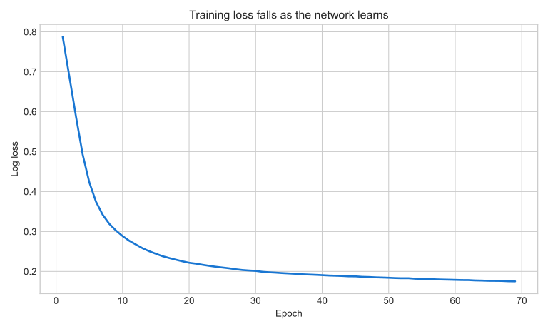
Lower log loss means the predicted probabilities became less wrong on the training batches. A falling curve is a useful training check, but it does not prove the model works on unseen data. Training loss can continue falling even while test performance gets worse.

Read Probabilities Before Labels

predict_proba() returns one probability for each class. For this binary target, column 0 is the probability of pass and column 1 is the probability of fail. The next step attaches the class-1 probability and final predicted label to five test rows.

failure_probability = model.predict_proba(X_test)[:, 1]
predicted_label = model.predict(X_test)

preview = X_test.head(5).copy()
preview["actual"] = y_test.head(5)
preview["failure_probability"] = failure_probability[:5].round(3)
preview["predicted"] = predicted_label[:5]

print(
    preview[[
        "motor_temperature_c",
        "vibration_mm_s",
        "hours_since_service",
        "actual",
        "failure_probability",
        "predicted",
    ]].to_string()
)

      motor_temperature_c  vibration_mm_s  hours_since_service  actual  failure_probability  predicted
331                  90.9            2.04                  153       0                0.000          0
1077                 65.1            1.90                  765       0                0.373          0
417                  72.8            2.98                  895       0                0.620          1
1175                 61.9            1.27                  262       0                0.000          0
932                  74.1            3.89                   12       0                0.000          0

Row 417 received a failure probability of 0.620, so the default 0.5 cutoff produced label 1. Its actual label was 0, making this a false alarm. Row 1077 stayed below the cutoff at 0.373 and was correctly labeled 0.

Probabilities contain more information than labels. A score of 0.51 and a score of 0.99 both become class 1, but they express very different levels of model confidence. They are model estimates, not guaranteed real-world risk values. Probability calibration would need a separate check before using them as operational risk scores.

Evaluate Errors on Unseen Rows

Accuracy alone is risky here. Because 87% of rows pass, a useless model that always predicts pass would already be about 87% accurate. A confusion matrix shows each kind of result instead.

from sklearn.metrics import classification_report, confusion_matrix

matrix = confusion_matrix(y_test, predicted_label)
print(matrix)
print(
    classification_report(
        y_test,
        predicted_label,
        target_names=["pass", "fail"],
        digits=3,
    )
)

[[199  10]
 [ 12  19]]
              precision    recall  f1-score   support

        pass      0.943     0.952     0.948       209
        fail      0.655     0.613     0.633        31

    accuracy                          0.908       240
   macro avg      0.799     0.782     0.790       240
weighted avg      0.906     0.908     0.907       240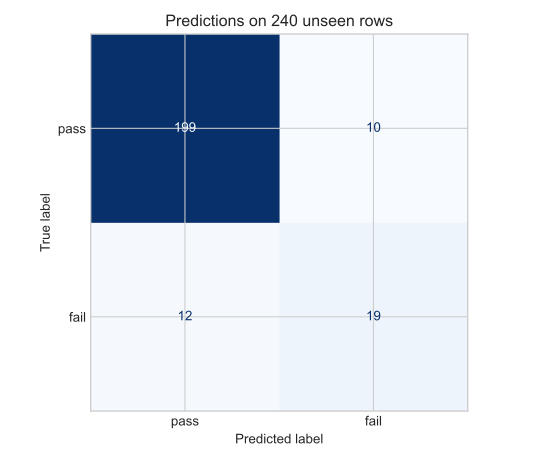

Read rows as actual classes and columns as predicted classes. The model correctly identified 199 passes and 19 failures. It raised 10 false alarms and missed 12 failures.

For the fail class, precision is 0.655: about 66% of predicted failures were actual failures. Recall is 0.613: the model found about 61% of all actual failures. The 0.908 accuracy sounds strong, but recall reveals an important weakness. In a real inspection system, missing 12 of 31 failures might be unacceptable. You could test a lower probability threshold to raise recall, but that would usually create more false alarms. The right trade-off depends on the cost of each error.

Common Mistakes and Troubleshooting

Training without scaling. An MLP updates many weights using numerical gradients. When columns have very different ranges, learning may be slow or unstable. Keep StandardScaler inside the pipeline so training and future predictions use the same transformation.

Scaling before the train/test split. A scaler fitted on all rows learns from the test distribution. Split first, then let the pipeline fit only on X_train.

Treating accuracy as the full result. This dataset has far more passes than failures. Always inspect the confusion matrix and the minority class’s precision and recall. Compare the model with a simple majority-class baseline.

Changing many settings at once. More layers do not automatically create a better model. Begin with one or two small hidden layers. Change one choice at a time, and compare it through cross-validation or a fixed validation plan.

Ignoring a convergence warning. If training reaches max_iter before stopping, first confirm that features are scaled. Then inspect the loss curve. You may need more epochs, a different learning rate, or simpler layers. Raising max_iter without checking the curve can hide the actual issue.

Expecting identical results without a seed. Initial weights, mini-batches, the train/test split, and the validation split include randomness. Set random_state when you need a reproducible lesson or experiment. Even with a seed, versions and hardware can cause small differences.

Using synthetic results as proof of real performance. This dataset is useful because its full generation process is known and reproducible. It does not contain sensor faults, maintenance practices, measurement errors, or changing conditions from a real facility. A production project needs representative real data, domain review, and monitoring after deployment.

Recap and a Safe Next Step

A small tabular neural network follows a clear sequence:

• Split the data first and stratify an imbalanced classification target.
• Put StandardScaler and MLPClassifier in one pipeline to prevent leakage and keep prediction preprocessing consistent.
• Use a small hidden-layer design, fixed random seed, and early stopping as a practical starting point.
• Inspect probabilities to understand how labels are formed.
• Evaluate the untouched test set with a confusion matrix, precision, and recall—not accuracy alone.

The durable mental model is “weighted combinations, non-linear activation, error, then weight updates.” Layers make those combinations flexible, but careful data handling and evaluation still decide whether the result is useful.

As a next experiment, lower the classification threshold from 0.5 to 0.35 and recompute the confusion matrix. Record how many additional failures are found and how many extra false alarms appear. That exercise connects the network’s probability output to a real decision trade-off without changing or retraining the model.