Build a Neural Network from Scratch with NumPy

A neural-network library can train a model in a few lines. That is useful, but the short code can hide the main idea: training is repeated array arithmetic. Values move forward to produce a prediction. Information about the prediction error moves backward to show how each weight should change.

This tutorial opens that process. We will build a small binary classifier using NumPy, not a machine-learning framework. It predicts whether a fictional water pump needs inspection from five sensor and service features. Binary classification means choosing between two outcomes, represented here by 0 and 1.

The goal is understanding, not replacing a tested framework in production. If features, labels, training sets, and test sets are new terms, start with your first machine learning model. That lesson explains the wider workflow before you implement an algorithm yourself.

Setup and prerequisites

You should know basic Python functions and have seen a two-dimensional NumPy array. You do not need calculus. We will describe every derivative by the job it performs.

Create a virtual environment, activate it, and install the three packages used in the lesson. The activation command below is for macOS and Linux; on Windows, use .venv\Scripts\activate instead.

python -m venv .venv
source .venv/bin/activate
python -m pip install numpy pandas matplotlib

The executed results in this article use Python 3.13.2, NumPy 2.5.1, pandas 3.0.3, and Matplotlib 3.11.0. The complete synthetic dataset is available as pump_inspection_readings.csv.

This dataset contains 1,200 fictional pump observations. It was created for this tutorial with NumPy’s recommended default_rng constructor and fixed seed 73. It is released as CC0-1.0. The readings are teaching data, not measurements from real pumps.

Load the file with pandas and inspect the first three rows:

import pandas as pd

pumps = pd.read_csv("pump_inspection_readings.csv")
print(pumps.head(3).to_string(index=False))
print("shape:", pumps.shape)
print("inspection labels:", pumps["needs_inspection"].value_counts().to_dict())

 inlet_pressure_kpa  motor_current_a  vibration_mm_s  bearing_temp_c  hours_since_service  needs_inspection
              271.73            19.19            1.68           55.84               1589.6                 1
              337.23            17.84            1.27           64.30                829.8                 0
              296.64            20.70            0.78           50.28                743.0                 0
shape: (1200, 6)
inspection labels: {0: 945, 1: 255}

Each row has five input features, such as pressure and temperature. needs_inspection is the label, or answer we want to predict. There are fewer positive labels than negative labels. We will therefore examine recall as well as accuracy later.

The mental model: four array transformations

Our network has five input values, one hidden layer with eight units, and one output. A unit is a small calculation that combines its inputs using learned weights. We can write the shape as 5 → 8 → 1.

One pass through the network has four stages:

1. Multiply each five-feature row by the first weight matrix and add a bias.
2. Apply ReLU to the eight hidden values. ReLU, short for rectified linear unit, keeps positive values and replaces negative values with zero.
3. Multiply the hidden values by a second weight matrix and add another bias.
4. Apply sigmoid, which changes the final number into a value between zero and one.

That final value is the model’s inspection score: a number between zero and one. It is not automatically a calibrated real-world probability. Training measures how wrong the scores are and sends correction signals backward. Backpropagation calculates how sensitive the loss is to each weight. Gradient descent uses those results to take a small step toward lower loss.

Here are the important shapes for 900 training rows:

X_train        (900, 5)
W1             (5, 8)
hidden         (900, 8)
W2             (8, 1)
probability    (900, 1)

The inner sizes match for each matrix product. NumPy’s @ operator follows matmul rules. For example, (900, 5) @ (5, 8) produces (900, 8).

Split and standardize the data

First, separate features from labels. Then shuffle row indices with a second fixed random seed and reserve 300 rows for the final test. The network never uses those rows to update its weights.

import numpy as np

feature_names = [
    "inlet_pressure_kpa",
    "motor_current_a",
    "vibration_mm_s",
    "bearing_temp_c",
    "hours_since_service",
]
X = pumps[feature_names].to_numpy(dtype=float)
y = pumps[["needs_inspection"]].to_numpy(dtype=float)

split_rng = np.random.default_rng(74)
indices = split_rng.permutation(len(X))
train_indices, test_indices = indices[:900], indices[900:]

X_train_raw, X_test_raw = X[train_indices], X[test_indices]
y_train, y_test = y[train_indices], y[test_indices]
print(X_train_raw.shape, X_test_raw.shape)

(900, 5) (300, 5)

Pressure is measured in hundreds, while vibration is often below five. Large differences in feature scale make gradient steps difficult to control. We will standardize each column by subtracting its training mean and dividing by its training standard deviation.

means = X_train_raw.mean(axis=0, keepdims=True)
stds = X_train_raw.std(axis=0, keepdims=True)

X_train = (X_train_raw - means) / stds
X_test = (X_test_raw - means) / stds

print("training means:", X_train.mean(axis=0).round(6))
print("training stds: ", X_train.std(axis=0).round(6))

training means: [-0.  0. -0.  0.  0.]
training stds:  [1. 1. 1. 1. 1.]

The tiny negative zeros are floating-point values rounded for display. The important result is that every training feature is centered near zero and has standard deviation one.

Notice that X_test uses the training means and standard deviations. Calculating new statistics from the test set would let information from the final evaluation affect preprocessing. Current scikit-learn documentation describes the same rule: learn scaling statistics from training samples, then reuse them for later data in StandardScaler.

Implement forward propagation

Start with sigmoid. Very large positive or negative inputs can make the exponential calculation overflow. np.clip limits those inputs before np.exp; the NumPy clip documentation defines this as limiting values to interval edges.

def sigmoid(values):
    clipped = np.clip(values, -30.0, 30.0)
    return 1.0 / (1.0 + np.exp(-clipped))

Next, create the four parameter arrays. A weight controls the strength and direction of a connection. A bias lets a unit shift its result instead of being fixed around zero. The random weights start small, while biases start at zero.

model_rng = np.random.default_rng(75)
params = {
    "W1": model_rng.normal(0, np.sqrt(2 / 5), (5, 8)),
    "b1": np.zeros((1, 8)),
    "W2": model_rng.normal(0, np.sqrt(2 / 8), (8, 1)),
    "b2": np.zeros((1, 1)),
}

Now express the forward pass directly from the mental model. Keep the intermediate arrays because backpropagation needs them.

def forward(X, params):
    hidden_linear = X @ params["W1"] + params["b1"]
    hidden = np.maximum(0.0, hidden_linear)
    probability = sigmoid(hidden @ params["W2"] + params["b2"])
    return hidden_linear, hidden, probability

hidden_linear, hidden, initial_probability = forward(X_train, params)
print(hidden.shape, initial_probability.shape)
print(initial_probability[:3].round(3).ravel())

(900, 8) (900, 1)
[0.305 0.364 0.555]

These are untrained scores. Random initial weights produce different values, but the scores do not yet represent useful inspection risk.

Measure error with binary cross-entropy

The model needs one number that summarizes how wrong all predictions are. Binary cross-entropy gives a large penalty when the model assigns a low score to a positive label or a high score to a negative label. Lower is better.

def binary_cross_entropy(y, probability):
    safe_probability = np.clip(probability, 1e-9, 1 - 1e-9)
    row_losses = (
        y * np.log(safe_probability)
        + (1 - y) * np.log(1 - safe_probability)
    )
    return float(-np.mean(row_losses))

initial_loss = binary_cross_entropy(y_train, initial_probability)
print(f"initial loss: {initial_loss:.6f}")

initial loss: 0.645671

Clipping here avoids log(0), which is undefined. This does not improve the predictions. It only keeps the loss calculation numerically safe.

Send the error backward

Backpropagation applies the chain rule from calculus, but each line has a practical meaning. For sigmoid combined with binary cross-entropy, the derivative at the output simplifies to probability - y. We divide by the row count because the loss is a mean.

def gradients(X, y, params):
    hidden_linear, hidden, probability = forward(X, params)
    rows = len(X)

    output_error = (probability - y) / rows
    grads = {
        "W2": hidden.T @ output_error,
        "b2": output_error.sum(axis=0, keepdims=True),
    }

    hidden_error = (
        output_error @ params["W2"].T
    ) * (hidden_linear > 0)
    grads["W1"] = X.T @ hidden_error
    grads["b1"] = hidden_error.sum(axis=0, keepdims=True)
    return grads

hidden_linear > 0 represents the ReLU derivative. It passes a correction through positions where ReLU kept a positive value and blocks it where ReLU produced zero. The matrix products then calculate a gradient for every weight.

Backpropagation code can run without raising an error even when one sign or transpose is wrong. A gradient check compares one analytic gradient with a numerical slope. Move one weight a very small distance in both directions, measure the two losses, and estimate the slope between them.

analytic = gradients(X_train[:32], y_train[:32], params)["W1"][0, 0]
epsilon = 1e-5
original = params["W1"][0, 0]

params["W1"][0, 0] = original + epsilon
loss_plus = binary_cross_entropy(y_train[:32], forward(X_train[:32], params)[2])
params["W1"][0, 0] = original - epsilon
loss_minus = binary_cross_entropy(y_train[:32], forward(X_train[:32], params)[2])
params["W1"][0, 0] = original

numeric = (loss_plus - loss_minus) / (2 * epsilon)
print(f"analytic: {analytic:.8f}")
print(f"numeric:  {numeric:.8f}")
print(f"difference: {abs(analytic - numeric):.2e}")

analytic: -0.01969722
numeric:  -0.01969722
difference: 1.95e-12

The difference is close to zero, so this tested parameter supports the implementation. One check does not prove that every line is correct, but it is a strong debugging tool. A larger project should sample several weights from every parameter matrix.

Train with gradient descent

Training repeats two actions: calculate gradients, then subtract a small fraction of each gradient from its parameter. One complete pass over the training rows is an epoch. This simple implementation uses all 900 rows in every update.

learning_rate = 0.08
epochs = 2_500

for epoch in range(epochs):
    grads = gradients(X_train, y_train, params)
    for name in params:
        params[name] -= learning_rate * grads[name]

final_training_probability = forward(X_train, params)[2]
final_training_loss = binary_cross_entropy(y_train, final_training_probability)
print(f"initial loss: {initial_loss:.6f}")
print(f"final training loss: {final_training_loss:.6f}")

initial loss: 0.645671
final training loss: 0.435194

The loss fell by about 0.21. That tells us the updates reduced the model’s error on the training rows. It does not yet tell us how the network handles unseen rows.

Evaluate held-out predictions

Run the 300 test rows forward once. We will label a pump for inspection when its score is at least 0.35.

test_probability = forward(X_test, params)[2]
test_prediction = (test_probability >= 0.35).astype(int)

truth = y_test.astype(int)
tn = int(((truth == 0) & (test_prediction == 0)).sum())
fp = int(((truth == 0) & (test_prediction == 1)).sum())
fn = int(((truth == 1) & (test_prediction == 0)).sum())
tp = int(((truth == 1) & (test_prediction == 1)).sum())

accuracy = (tp + tn) / len(y_test)
precision = tp / (tp + fp)
recall = tp / (tp + fn)
print(f"test loss: {binary_cross_entropy(y_test, test_probability):.6f}")
print(f"accuracy:  {accuracy:.3f}")
print(f"precision: {precision:.3f}")
print(f"recall:    {recall:.3f}")
print([[tn, fp], [fn, tp]])

test loss: 0.434506
accuracy:  0.790
precision: 0.508
recall:    0.484
[[206, 30], [33, 31]]

The test loss is close to the training loss, so this run shows no large train-test loss gap. Accuracy says 79% of all test labels were correct. Precision says about 51% of inspection flags matched a positive label. Recall says the model found about 48% of pumps that had a positive label.

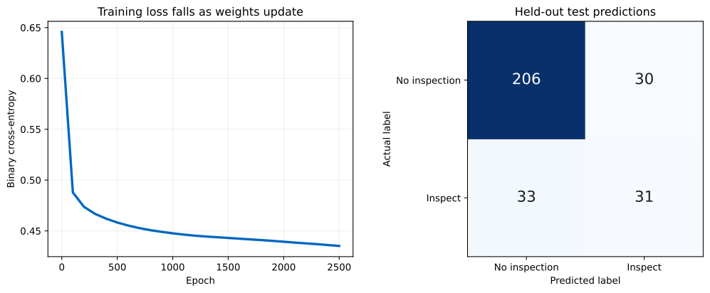
The left panel confirms that weight updates steadily reduced training loss. The right panel separates the four test outcomes. The 33 false negatives matter because they are pumps that needed inspection but were not flagged.

The 0.35 threshold is a decision rule chosen for this example, not a value learned by the training loop. Raising it usually reduces false positives but misses more positive cases. Lowering it usually catches more positives but sends more pumps for unnecessary inspection. In a real project, choose the threshold with separate validation data and explicit cost information, then evaluate once on untouched test data.

Common mistakes and troubleshooting

Matrix multiplication reports a shape error. Print every shape and compare adjacent inner dimensions. X @ W1 requires the feature count in X to equal the first dimension of W1. Keep labels shaped (rows, 1) so they match the output.

Loss becomes nan. Check feature scaling, reduce the learning rate, and clip inputs to exp and log. A very large learning rate can make weights grow until floating-point arithmetic becomes unstable.

Loss stays almost unchanged. Confirm that parameter updates use subtraction, not addition. Check that learning_rate is not extremely small. Run a numerical gradient check before changing the architecture.

The test set was standardized separately. Do not call mean and std on test or future rows. Store the training statistics and reuse them in the same feature order.

Accuracy looks good while positive cases are missed. This dataset has 945 negative rows and 255 positive rows. A model can gain high accuracy by favoring the common class. Always inspect the confusion matrix, precision, and recall.

A score is treated as a calibrated probability or guarantee. Sigmoid keeps the output between zero and one, but that alone does not prove that a score such as 0.70 corresponds to a 70% real-world event rate. This lesson’s fictional dataset cannot support real maintenance decisions.

The same seed gives different rows after a library upgrade. A seed makes a run reproducible within the tested environment. NumPy notes that Generator does not promise an identical bit stream across all future versions. Vendor the generated CSV when exact long-term rows matter.

This code is moved directly into production. The implementation leaves out mini-batches, regularization, early stopping, model persistence, automated differentiation, and many numerical checks. Use it to understand the mechanism. Use a maintained framework for systems that affect people, money, safety, or operations.

Recap

A small neural network is a sequence of understandable array operations:

• Standardize features with statistics learned only from training data.
• Multiply inputs by weights, add biases, and apply ReLU in the hidden layer.
• Apply sigmoid at the output to produce a score between zero and one.
• Use binary cross-entropy to measure prediction error.
• Backpropagate that error to calculate one gradient per parameter.
• Subtract a small gradient step repeatedly until training loss falls.
• Check gradients numerically and evaluate on rows that never updated the weights.
• Read a confusion matrix and choose a decision threshold for the real cost of errors.

The durable mental model is forward to predict, compare to measure error, backward to assign correction, update to learn. Once those four stages are clear, a framework’s short training API becomes easier to reason about and debug.