NumPy Broadcasting for Column-Wise Standardization

A greenhouse records temperature, humidity, and carbon dioxide every two hours. These measurements cannot be compared directly: temperature is near 20, humidity is near 70, and carbon dioxide is near 600. Because the units differ, one column can look numerically larger even when its readings are not more unusual.

We can put each feature on a comparable scale with standardization. Standardization subtracts a column’s mean and divides by that column’s standard deviation. The result is a z-score, which says how many standard deviations a value is above or below its column mean.

Doing this to a whole matrix is a practical way to learn broadcasting. Broadcasting is NumPy’s rule for applying an operation to arrays with compatible shapes without manually copying values. By the end, you will know how to read those shapes, preserve useful dimensions, and fix the common error operands could not be broadcast together.

If arrays themselves are new to you, the examples in Python data structures provide useful background before you continue.

Prerequisites and setup

You need Python 3.10 or later and basic experience running a Python file or notebook cell. An array is a grid of values. A two-dimensional array has rows and columns, and its shape reports their sizes as (rows, columns).

Create an isolated environment and install the packages used in this lesson. On macOS or Linux, run:

python -m venv .venv
source .venv/bin/activate
python -m pip install numpy pandas matplotlib

On Windows PowerShell, replace the activation command with .venv\Scripts\Activate.ps1.

The executed results use Python 3.13.2, NumPy 2.5.1, pandas 3.0.3, and Matplotlib 3.11.0. Download the synthetic greenhouse readings and save the file as greenhouse_readings.csv.

This dataset was created for this tutorial and is released under CC0-1.0. Every time and sensor reading is fictional. It contains no readings from a real greenhouse.

Start with the matrix and its shape

First, load the CSV with pandas. Keep the time labels in the pandas table, then select the three numeric features and convert them into a NumPy array:

import numpy as np
import pandas as pd

readings = pd.read_csv("greenhouse_readings.csv")
feature_names = ["temperature_c", "humidity_pct", "co2_ppm"]
values = readings[feature_names].to_numpy(dtype=float)

print(readings.to_string(index=False))
print("values shape:", values.shape)

 time  temperature_c  humidity_pct  co2_ppm
08:00           18.2            78      510
10:00           20.1            72      545
12:00           23.4            61      620
14:00           25.0            55      690
16:00           22.8            63      640
18:00           19.7            71      560
values shape: (6, 3)

The shape (6, 3) means six observation rows and three feature columns. Shape is more important than the variable name when you reason about broadcasting. NumPy sees dimensions, not concepts such as “time” or “sensor.”

The three columns also have different units. A difference of 50 ppm in carbon dioxide is not directly comparable with a difference of 5 degrees Celsius. We need one center and one scale for each column.

Mental model: compare shapes from the right

NumPy compares two shapes from their rightmost dimensions. A pair of dimensions is compatible when either:

• the sizes are equal, or
• one size is 1.

If one shape has fewer dimensions, imagine adding dimensions of size 1 on its left. NumPy applies this check dimension by dimension. The current NumPy broadcasting guide describes the same rule for element-wise operations.

For our matrix, a row-shaped set of three statistics is compatible:

values:       (6, 3)
column stats: (1, 3)
               |  |
               |  +-- 3 matches 3
               +----- 1 can expand across 6 rows
result:       (6, 3)

“Expand” is a way to understand the operation. NumPy does not need us to create six physical copies of the statistics row. It behaves as if that row were available beside every observation.

You can ask NumPy to check the result shape before doing arithmetic:

print(np.broadcast_shapes((6, 3), (1, 3)))

(6, 3)

This is useful when a long calculation contains several arrays. Check the shapes first, then inspect the values.

Keep the column dimension during aggregation

We need the mean and standard deviation of each column. axis=0 tells NumPy to aggregate down the rows, leaving one result per column. The option keepdims=True preserves the reduced row axis with size 1:

column_means = values.mean(axis=0, keepdims=True)
column_stds = values.std(axis=0, keepdims=True)

print("mean shape:", column_means.shape)
print("means:", np.round(column_means, 3))
print("standard deviations:", np.round(column_stds, 3))

mean shape: (1, 3)
means: [[ 21.533  66.667 594.167]]
standard deviations: [[ 2.368  7.717 61.401]]

Each position belongs to the column at the same position: 21.533 is the temperature mean, 66.667 is the humidity mean, and 594.167 is the carbon dioxide mean.

Without keepdims=True, the means would have shape (3,). That one-dimensional shape also broadcasts correctly against (6, 3) because its three positions align with the matrix’s rightmost dimension. Keeping (1, 3) is still helpful because it makes “one row of column statistics” visible. NumPy’s current std documentation also notes that retained dimensions broadcast correctly against the input.

We use NumPy’s default ddof=0, so the code calculates population standard deviation for these six values. This lesson treats the CSV as the complete fictional day we want to transform. If the rows were a sample used to estimate a larger population, you might choose ddof=1; document that choice because it changes the result.

Standardize every column in one expression

Now apply the z-score formula. Both the subtraction and division use broadcasting. The (1, 3) mean row and standard-deviation row each align with all six rows of the (6, 3) matrix:

standardized = (values - column_means) / column_stds

print("result shape:", standardized.shape)
print(np.round(standardized, 3))

result shape: (6, 3)
[[-1.408  1.469 -1.371]
 [-0.605  0.691 -0.801]
 [ 0.788 -0.734  0.421]
 [ 1.464 -1.512  1.561]
 [ 0.535 -0.475  0.746]
 [-0.774  0.562 -0.556]]

Read the first row by column. At 08:00, temperature is 1.408 standard deviations below its daily mean. Humidity is 1.469 standard deviations above its mean. Carbon dioxide is 1.371 standard deviations below its mean. The values now share a unit-free scale, but each sign and distance still refers to its own column.

The fourth row shows a different pattern. At 14:00, temperature and carbon dioxide are both more than one standard deviation above their means, while humidity is more than one standard deviation below its mean. Standardization makes that cross-feature pattern easier to see; it does not prove that one sensor caused another to change.

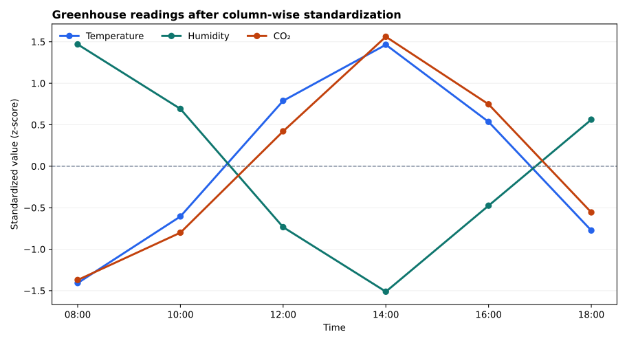
The dashed zero line represents each feature’s own mean. A point above zero is above that column’s mean, and a point below zero is below it. The chart is generated from the same standardized matrix shown in the output.

Verify the transformation instead of trusting it

A correct standardized column has mean 0 and population standard deviation 1, apart from tiny floating-point rounding differences. Calculate both checks down the rows:

check_means = standardized.mean(axis=0)
check_stds = standardized.std(axis=0)

print("column means:", np.round(check_means, 12))
print("column standard deviations:", np.round(check_stds, 12))

column means: [ 0. -0.  0.]
column standard deviations: [1. 1. 1.]

The displayed -0. is not a negative measurement. It is a very small negative floating-point result rounded to zero. For an automated check, use np.allclose with a tolerance instead of exact equality:

assert np.allclose(check_means, 0.0, atol=1e-12)
assert np.allclose(check_stds, 1.0, atol=1e-12)

These checks test the intended property, not only the output shape. A calculation can produce a (6, 3) matrix and still use the wrong axis.

A shape error and how to repair it

Suppose you reshape the three means as a column vector instead of a row vector:

wrong_means = values.mean(axis=0)[:, np.newaxis]
print("wrong mean shape:", wrong_means.shape)
values - wrong_means

wrong mean shape: (3, 1)
ValueError: operands could not be broadcast together with shapes (6,3) (3,1)

Compare the dimensions from the right. The last dimensions 3 and 1 are compatible. The next dimensions 6 and 3 are neither equal nor 1, so the operation fails. A (3, 1) vector is arranged as three rows, but our three statistics describe columns.

Repair it by keeping the aggregation dimension:

right_means = values.mean(axis=0, keepdims=True)
print(right_means.shape)

(1, 3)

Do not add or remove axes until the code stops raising an error. Write what each axis means, print every relevant shape, and make the layout match that meaning.

Common mistakes and troubleshooting

Using axis=1 for column statistics. axis=1 reduces the columns and returns one statistic per row. For one statistic per feature column, reduce the row axis with axis=0.

Standardizing a label column. Convert only numeric feature columns to the NumPy array. A time string is an identifier here, not a measurement to standardize.

Dividing by zero. A constant column has a standard deviation of zero. After subtracting its mean, the z-score calculation divides zero by zero and produces nan. Detect constant columns first with column_stds == 0. You can remove the constant feature, leave it unchanged, or define a project-specific rule.

Assuming broadcasting matches by column name. NumPy aligns positions and shapes, not pandas labels. If feature order changes, a statistics array may be applied to the wrong feature while shapes still look valid. Keep a stable feature_names list and use it for both fitting and later transformation.

Calculating statistics separately on future data. In a machine-learning workflow, calculate means and standard deviations on the training set, then reuse those same values for validation, test, and new observations. Recalculating them leaks information and changes the scale.

Using exact equality for floating-point checks. Arithmetic can leave tiny residuals such as -2e-16. Use np.allclose with a suitable tolerance.

Materializing repeated rows. Functions such as np.tile can create a larger array of repeated statistics. Broadcasting expresses the intended element-wise operation directly and usually avoids that unnecessary allocation.

Recap

NumPy broadcasting is easiest to reason about through shapes:

1. Write the shapes and compare dimensions from right to left.
2. Two dimensions work together when they are equal or one is 1.
3. Use axis=0 to calculate one statistic per matrix column.
4. Use keepdims=True when a visible singleton dimension makes the intended alignment clearer.
5. Verify the mathematical property after the operation, not only the output shape.

For this greenhouse matrix, (6, 3) combined with (1, 3) to produce (6, 3). One row of means and one row of standard deviations applied across six observations. That same pattern appears in feature scaling, image processing, simulation, and many machine-learning calculations: give each axis a clear meaning, preserve the dimensions you need, and let compatible shapes do the repeated work.