How to Calculate Paired Effect Size in Python with Bootstrap

One reviewer needs 52.5 minutes to check a spreadsheet with the old checklist and 50.4 minutes with the new one. That difference is 2.1 minutes, but the dataset contains 36 reviewers. Some improve much more, while others take longer. One pair cannot describe the overall change.

To calculate a paired effect size in Python, subtract each unit’s after value from its matching before value. Divide the mean of those differences by their sample standard deviation to get Cohen’s dz, and bootstrap the differences to show uncertainty around both the raw and standardized results.

This tutorial applies that workflow to fictional review times. It answers a before-and-after question, not a comparison between two independent teams. You will keep every pair intact, inspect individual changes, and avoid turning one standardized number into a causal claim.

Prerequisites and setup

You need Python 3.10 or later and basic experience running a Python file or notebook cell. A pandas DataFrame is a table with named rows and columns. NumPy calculates the statistics, SciPy creates the bootstrap intervals, and Matplotlib draws the chart. You do not need previous experience with effect sizes or resampling.

Create a virtual environment and install the four packages used in the lesson. On macOS or Linux, run:

python -m venv .venv
source .venv/bin/activate
python -m pip install numpy pandas scipy matplotlib

On Windows PowerShell, activate the environment with .venv\Scripts\Activate.ps1. The published results were executed with Python 3.13.2, NumPy 2.5.1, pandas 3.0.3, SciPy 1.18.0, and Matplotlib 3.11.0.

Download the synthetic review-time CSV and save it beside your Python file. The dataset is original fictional teaching data released under CC0-1.0. Its 36 reviewer IDs and times do not describe real people, software, or an organization.

The final chart is an SVG file. Select Matplotlib’s non-interactive Agg backend before importing pyplot so the same code can save the chart on a server without a desktop:

import matplotlib

matplotlib.use("Agg")

import matplotlib.pyplot as plt
import numpy as np
import pandas as pd
from scipy.stats import bootstrap

Understanding change within pairs

Data is paired when two measurements belong to the same unit. Here, the unit is a reviewer. RV-001 before the checklist change must stay with RV-001 afterward.

The analysis therefore starts with a difference within each row, not with separate summaries of the two columns:

minutes saved = before minutes - after minutes

A positive result means the review became faster. A negative result means it became slower. This direction is a choice, so state it before calculating anything.

The raw mean change stays in minutes, which makes it easy to use. A standardized effect divides that mean by a standard deviation. For paired data, this tutorial uses Cohen’s dz:

Cohen's dz = mean of paired differences / sample SD of paired differences

The z label matters. Several standardized effect-size formulas exist for repeated measurements, and they use different denominators. Cohen’s dz uses the spread of the difference scores. The calculation and its paired-sample role are described in this practical effect-size primer.

This denominator answers a specific question: how large is the average change compared with the reviewer-to-reviewer variation in change? It does not convert minutes into a universal measure of practical value. For that reason, report minutes first and dz second.

Load the data and protect the pairs

Start by loading the CSV and viewing six rows. Small previews make the pairing visible before a summary hides it.

reviews = pd.read_csv("review_time_before_after.csv")
print(reviews.head(6).to_string(index=False))
print("shape:", reviews.shape)

reviewer_id  before_minutes  after_minutes
     RV-001            52.5           50.4
     RV-002            50.9           46.5
     RV-003            45.8           43.5
     RV-004            42.6           31.6
     RV-005            52.1           57.1
     RV-006            33.0           23.1
shape: (36, 3)

Each row contains one complete pair. The fifth row is important: RV-005 takes longer after the change. A valid analysis keeps that result instead of deleting it because it moves against the average.

Now check that every ID occurs once and every required cell is present. These checks stop the program early if a join duplicated a reviewer or a measurement is missing.

required = ["reviewer_id", "before_minutes", "after_minutes"]

assert reviews["reviewer_id"].is_unique
assert not reviews[required].isna().any().any()

print("unique reviewer IDs:", reviews["reviewer_id"].nunique())
print("missing required values:", int(reviews[required].isna().sum().sum()))

unique reviewer IDs: 36
missing required values: 0

If one side of a pair is missing, do not calculate each column from a different set of reviewers. Investigate the missing value or remove the whole incomplete pair and report that choice.

Calculate the raw change first

Create one difference per reviewer using the direction defined earlier. The source values have one decimal place, so round each difference to the same precision. Then summarize the before values, after values, and differences.

reviews["minutes_saved"] = (
    reviews["before_minutes"] - reviews["after_minutes"]
).round(1)

differences = reviews["minutes_saved"].to_numpy()

print(f"mean before: {reviews['before_minutes'].mean():.2f} minutes")
print(f"mean after: {reviews['after_minutes'].mean():.2f} minutes")
print(f"mean saved: {differences.mean():.2f} minutes")
print(f"median saved: {np.median(differences):.2f} minutes")
print(
    "faster / slower / unchanged:",
    int((differences > 0).sum()), "/",
    int((differences < 0).sum()), "/",
    int((differences == 0).sum()),
)

mean before: 46.49 minutes
mean after: 44.11 minutes
mean saved: 2.37 minutes
median saved: 2.85 minutes
faster / slower / unchanged: 25 / 11 / 0

The average falls by 2.37 minutes, and the median reviewer saves 2.85 minutes. However, 11 of the 36 reviewers become slower. The mean is a useful group summary, but it is not a claim that every reviewer benefits.

The raw result should remain the main result because minutes have direct meaning. If saving two minutes is too small to affect a decision, a standardized label cannot make it useful.

Standardize the mean with Cohen’s dz

Next, turn the formula into a small function. ddof=1 asks NumPy for the sample standard deviation. NumPy’s std documentation explains that its default is ddof=0, so the sample choice must be explicit.

def cohens_dz(values, axis=-1):
    standard_deviation = np.std(values, axis=axis, ddof=1)
    if np.any(standard_deviation == 0):
        raise ValueError("Cohen's dz is undefined when every change is identical.")
    return np.mean(values, axis=axis) / standard_deviation


change_sd = np.std(differences, ddof=1)
effect_size = cohens_dz(differences)

print(f"sample SD of changes: {change_sd:.2f} minutes")
print(f"Cohen's dz: {effect_size:.3f}")

sample SD of changes: 4.50 minutes
Cohen's dz: 0.528

The positive sign follows our definition of saved time. The average saving is 0.528 standard deviations of the observed changes. This gives scale-free context, but it should not be read as 0.528 minutes or as the percentage of reviewers who improve.

You may see fixed labels such as small, medium, and large attached to Cohen’s d. Treat them as rough context, not automatic decisions. The same standardized value can matter differently for a medical measure, a processing time, or a model score. The raw 2.37-minute change and the count of 25 faster versus 11 slower reviewers provide information that dz alone cannot show.

If you need a refresher on why sample and population standard deviations differ, see our descriptive statistics guide.

Add bootstrap confidence intervals

The observed data gives one estimate. A bootstrap repeatedly samples the 36 difference scores with replacement and recalculates the statistic. “With replacement” means one reviewer’s difference may appear more than once in a resample while another may be absent.

Because we already reduced each pair to one difference, resampling differences keeps the pair structure intact. The next call estimates uncertainty around the mean saving. We request 20,000 resamples, set a fixed random generator for reproducibility, and choose the bias-corrected and accelerated (BCa) method. BCa adjusts the interval endpoints for bias and skewness in the bootstrap estimates.

mean_result = bootstrap(
    (differences,),
    np.mean,
    confidence_level=0.95,
    n_resamples=20_000,
    method="BCa",
    rng=np.random.default_rng(5812),
)

mean_low = mean_result.confidence_interval.low
mean_high = mean_result.confidence_interval.high
print(f"95% BCa interval for mean change: {mean_low:.2f} to {mean_high:.2f} minutes")

95% BCa interval for mean change: 0.96 to 3.82 minutes

SciPy’s current bootstrap documentation defines the rng argument for repeatable behavior and returns both a confidence interval and a bootstrap distribution. It also warns that BCa can fail on degenerate data, such as a sample in which every value is identical.

Under this resampling procedure, the 95% confidence interval for the population mean change runs from about 0.96 to 3.82 minutes. It describes uncertainty from sampling reviewers like those represented here. It does not mean that 95% of individual reviewers save between those two values, and it does not account for a biased or unrealistic sample.

Use the same method for dz. The function already accepts an axis argument, so SciPy can calculate many resamples efficiently.

dz_result = bootstrap(
    (differences,),
    cohens_dz,
    confidence_level=0.95,
    n_resamples=20_000,
    method="BCa",
    rng=np.random.default_rng(5813),
)

dz_low = dz_result.confidence_interval.low
dz_high = dz_result.confidence_interval.high
print(f"95% BCa interval for dz: {dz_low:.2f} to {dz_high:.2f}")

95% BCa interval for dz: 0.18 to 0.88

The interval is wide compared with the point estimate of 0.528. Values near either end would lead to different judgments about practical importance. More bootstrap resamples make the numerical calculation smoother, but they do not create more reviewers or more representative data.

Read the individual and bootstrap views together

The generated chart preserves both levels of the result:

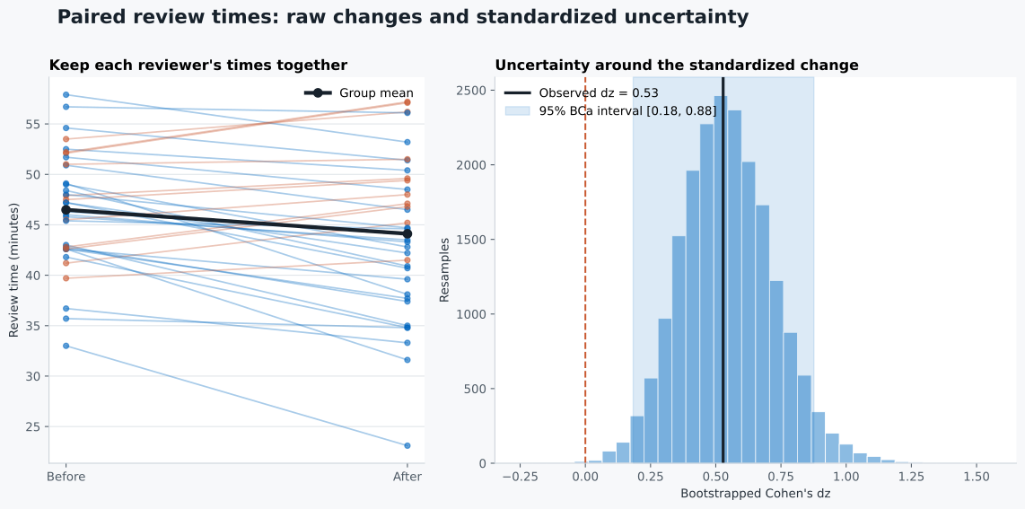
Read the left panel one line at a time. Blue falling lines are faster reviews, while orange rising lines are slower reviews. The thick black line shows the group mean. It falls, but the mixed individual directions warn against saying that the checklist helps everyone.

Read the right panel against zero. The vertical dark line marks the observed dz, and the shaded band marks its BCa interval. The distribution shows how much the standardized estimate changes across resamples of this small synthetic group.

This is a descriptive before-and-after example. It does not isolate the cause of the change. Reviewers may have improved through practice, the second spreadsheets may have been easier, or another process may have changed at the same time. A randomized or counterbalanced design would be needed for a stronger causal conclusion.

Common mistakes and troubleshooting

Treating the columns as independent groups. Do not shuffle, sort, or resample the before and after columns separately. Match on a stable ID and calculate one difference per unit.

Reversing the sign without noticing. before - after makes time savings positive. after - before is also valid, but improvements then become negative. Define the direction in words and use it consistently.

Deleting slower reviewers. Negative differences are valid observations unless a documented data-quality problem makes them invalid. Removing them only because they oppose the average biases the result.

Using the two column standard deviations in the denominator. Cohen’s dz uses the sample standard deviation of the paired differences. A pooled standard deviation belongs to a different effect-size definition and answers a different question.

Forgetting ddof=1. NumPy defaults to a population-style denominator. Pass ddof=1 when calculating the sample standard deviation used here.

Getting ValueError from cohens_dz. If every difference is identical, their standard deviation is zero, so division is undefined. Report the identical raw change and do not force a standardized value. With a small sample or only a few distinct differences, a bootstrap resample can also have zero spread; in that case, review whether BCa is suitable for the data.

Assuming the fixed seed proves stability. The seed makes this lesson reproducible. Try other seeds as a numerical check, but collect more representative pairs when you need less sampling uncertainty.

Calling the result causal. Pairing controls for stable differences between reviewers, but time order and other changes can still explain the result. Match the claim to the study design.

For experiments that compare independent groups and must be planned before data collection, continue with A/B test sample-size planning in Python.

What you learned

A paired effect-size workflow starts with identities, not averages. Keep each unit’s two measurements on one row, define the direction, and calculate one difference. Report the mean difference in the original units before standardizing it.

In this synthetic review exercise, the mean saving is 2.37 minutes and Cohen’s dz is 0.528. The 95% BCa intervals are 0.96 to 3.82 minutes for the mean change and 0.18 to 0.88 for dz. Those intervals show sampling uncertainty, while the 25 faster and 11 slower reviewers show variation that the average hides.

The durable rule is pair, subtract, summarize, then standardize. Keep the raw change, the standardized change, the uncertainty interval, and the study limits together so readers can judge both statistical scale and practical meaning.