How to Summarize Data with Pandas Pivot Tables

Someone on your team asks for “average score by office, broken out by quarter, with a total row at the bottom.” You could get there with groupby, some unstack()-ing, and a bit of manual total-row math — our post on Pandas groupby covers that path in full. Or you could reach for the one method built to answer exactly this shape of question in a single call: pivot_table.

DataFrame.pivot_table() builds that grid directly. Give it index for the row groups, columns for the column groups, values for the column to aggregate, and aggfunc for how to aggregate it (it defaults to the mean). Call survey.pivot_table(index="office", columns="quarter", values="score") and pandas splits the rows by office and quarter, averages the score within each combination, and lays the result out as a table — offices down the side, quarters across the top — with no separate reshaping step required.

Four Arguments, One Grid

Every pivot table you’ll ever build is the same four decisions:

• index — which column’s values become the rows.
• columns — which column’s values become the columns (optional; leave it out and you get a flat one-column-per-value summary instead of a grid).
• values — which column gets aggregated into each cell.
• aggfunc — what function turns a group of raw rows into that one cell ("mean" by default).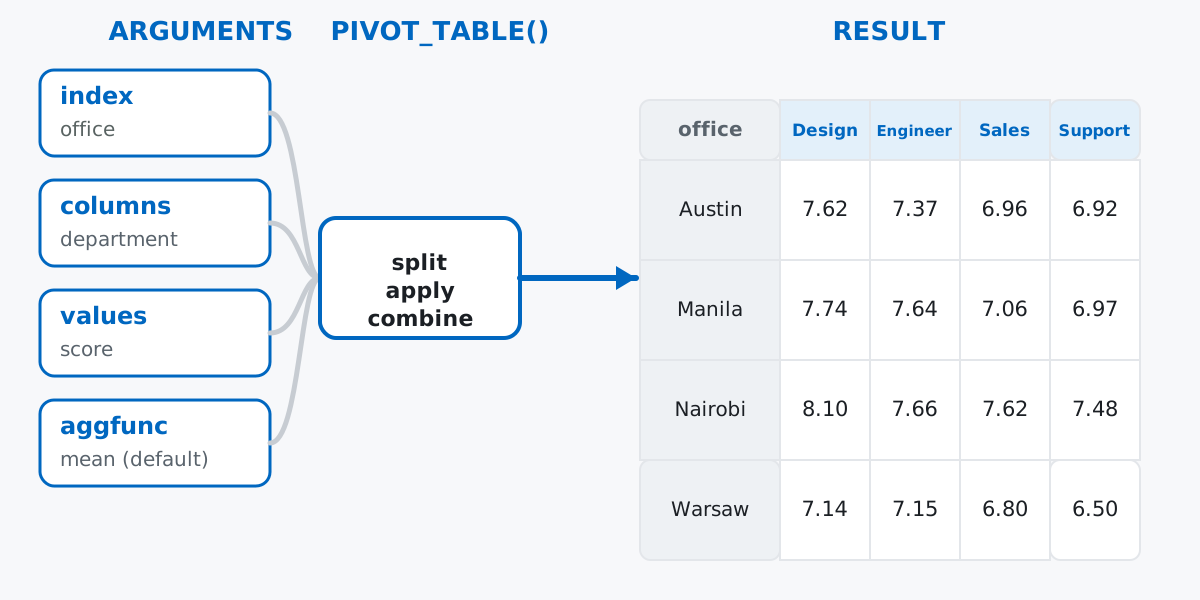

It’s the same split-apply-combine idea behind groupby — split the rows into groups, apply a function to each group, combine the results — except the combine step arranges everything into a two-dimensional grid instead of handing back a flat list. Once you can name which column plays each of those four roles, you can build the table, and everything below is really just different answers to “what do I put in aggfunc.”

961 Survey Responses, Four Offices, Two Years

Rather than hunting down a real happiness dataset with a license clear enough to republish, here’s a scenario you can regenerate exactly: a distributed company runs a quarterly wellbeing survey (a 0-10 satisfaction score, plus hours worked that week) across four offices and four departments. Austin, Nairobi, and Warsaw have been running the survey since early 2024; Manila opened partway through and joined in the third quarter.

import numpy as np
import pandas as pd

rng = np.random.default_rng(42)

offices = ["Austin", "Nairobi", "Warsaw", "Manila"]
departments = ["Engineering", "Sales", "Support", "Design"]
quarters = [f"{year}-Q{q}" for year in (2024, 2025) for q in (1, 2, 3, 4)]

office_base = {"Austin": 7.4, "Nairobi": 7.9, "Warsaw": 7.1, "Manila": 7.6}
dept_adjust = {"Engineering": 0.1, "Sales": -0.3, "Support": -0.5, "Design": 0.2}

rows = []
for office in offices:
    for quarter in quarters:
        if office == "Manila" and quarter < "2024-Q3":
            continue  # the Manila office didn't exist yet
        for dept in departments:
            n_resp = rng.integers(4, 13)
            mean = office_base[office] + dept_adjust[dept]
            scores = rng.normal(mean, 1.1, size=n_resp).clip(0, 10).round(1)
            hours = rng.normal(41, 4, size=n_resp).clip(30, 55).round(1)
            for score, hrs in zip(scores, hours):
                rows.append((office, dept, quarter, score, hrs))

survey = pd.DataFrame(rows, columns=["office", "department", "quarter", "score", "hours_per_week"])
survey.shape

(961, 5)

survey.head()

   office   department  quarter  score  hours_per_week
0  Austin  Engineering  2024-Q1    6.4            35.8
1  Austin  Engineering  2024-Q1    8.3            41.5
2  Austin  Engineering  2024-Q1    8.5            39.7
3  Austin  Engineering  2024-Q1    5.4            40.9
4  Austin        Sales  2024-Q1    6.2            40.8

961 rows, one per survey response. (The outputs below come from pandas 3.0 — everything shown also works on pandas 2.x.)

A Summary That’s Still a DataFrame

Start with a single grouping column and no columns argument — the simplest shape:

survey.pivot_table(index="office", values="score").round(2)

         score
office        
Austin    7.21
Manila    7.38
Nairobi   7.71
Warsaw    6.89

That number matches what survey.groupby("office")["score"].mean() would give you, but there’s a real difference in what comes back:

type(survey.groupby("office")["score"].mean())

<class 'pandas.Series'>

type(survey.pivot_table(index="office", values="score"))

<class 'pandas.DataFrame'>

groupby with a single column selected hands you a Series; pivot_table always hands you a DataFrame, even with one values column and no columns argument at all. That matters the moment you want to chain a second aggregation, rename a column, or merge the result back onto something else — a DataFrame gives you a column to address by name instead of a bare Series name.

Two Categories, One Grid

Add columns and the real shape of pivot_table shows up — a full cross-tab of office against department:

survey.pivot_table(index="office", columns="department", values="score").round(2)

department  Design  Engineering  Sales  Support
office                                         
Austin        7.62         7.37   6.96     6.92
Manila        7.74         7.64   7.06     6.97
Nairobi       8.10         7.66   7.62     7.48
Warsaw        7.14         7.15   6.80     6.50

Sixteen numbers, one glance. Every office reads slightly happier in Design and slightly lower in Support — worth a second look, but not this post’s job to explain. (The official pivot_table reference documents every argument shown here and a handful more, if you want the full signature.)

Empty Cells Mean No Data, Not Zero

Cross office against quarter instead of department, and the Manila gap shows up honestly:

survey.pivot_table(index="office", columns="quarter", values="score").round(2)

quarter  2024-Q1  2024-Q2  2024-Q3  2024-Q4  2025-Q1  2025-Q2  2025-Q3  2025-Q4
office                                                                         
Austin      7.27     7.20     7.06     6.87     7.30     7.31     7.30     7.31
Manila       NaN      NaN     7.46     7.28     7.24     7.47     7.67     7.20
Nairobi     7.77     7.89     7.48     7.78     7.67     7.94     7.69     7.47
Warsaw      7.06     6.71     7.17     6.58     7.24     7.03     6.70     6.63

NaN there is correct — Manila didn’t run the survey in 2024-Q1 or 2024-Q2, so there’s genuinely no score to average. If you need a table with no gaps — say, to count how many responses came in each quarter rather than average them — fill_value fills those missing cells, and a response count is a case where zero is actually true:

survey.pivot_table(index="office", columns="quarter", values="score", aggfunc="count", fill_value=0)

quarter  2024-Q1  2024-Q2  2024-Q3  2024-Q4  2025-Q1  2025-Q2  2025-Q3  2025-Q4
office                                                                         
Austin        34       38       38       29       35       39       31       30
Manila         0        0       26       36       39       36       33       29
Nairobi       36       29       24       33       34       29       33       33
Warsaw        36       30       29       29       26       32       29       26

Zero responses is a real, meaningful zero. An average score of zero would not be — filling the first table’s NaN cells with 0 would claim Manila’s employees rated their nonexistent early quarters as miserable as it gets, which is nonsense. Match fill_value to what “no data” actually means for the number you’re computing.

Two Statistics Per Cell

aggfunc takes a list just as happily as a single string, and the result grows an extra column level:

survey.pivot_table(index="office", columns="department", values="score", aggfunc=["mean", "count"]).round(2)

             mean                            count                          
department Design Engineering Sales Support Design Engineering Sales Support
office                                                                      
Austin       7.62        7.37  6.96    6.92     67          64    74      69
Manila       7.74        7.64  7.06    6.97     50          59    43      47
Nairobi      8.10        7.66  7.62    7.48     60          67    61      63
Warsaw       7.14        7.15  6.80    6.50     70          47    60      60

Now you can eyeball whether a striking average is backed by a real sample or a handful of responses — Manila’s Sales column, for instance, is averaging over only 43 responses, the smallest cell in the table.

Row and Column Totals with margins=True

Pass margins=True and pivot_table adds a total row and column, computed over the actual underlying rows rather than just averaging the cells you can already see:

survey.pivot_table(
    index="office", columns="department", values="score",
    aggfunc="mean", margins=True, margins_name="All Offices",
).round(2)

department   Design  Engineering  Sales  Support  All Offices
office                                                       
Austin         7.62         7.37   6.96     6.92         7.21
Manila         7.74         7.64   7.06     6.97         7.38
Nairobi        8.10         7.66   7.62     7.48         7.71
Warsaw         7.14         7.15   6.80     6.50         6.89
All Offices    7.62         7.48   7.11     6.97         7.30

That bottom-right corner — 7.30 — is the mean of every one of the 961 raw scores, not the average of the four row totals above it. With unequal group sizes those two numbers usually differ, even if only slightly here:

grid = survey.pivot_table(
    index="office", columns="department", values="score",
    aggfunc="mean", margins=True, margins_name="All Offices",
)
simple_average = grid.loc[["Austin", "Manila", "Nairobi", "Warsaw"], "All Offices"].mean()
true_grand_mean = grid.loc["All Offices", "All Offices"]
round(simple_average, 4), round(true_grand_mean, 4)

(7.298, 7.2972)

Manila has fewer total responses than the other three offices, so it pulls less weight in the true grand mean than a simple four-way average would give it. The gap is small in this dataset; with more lopsided group sizes it stops being a rounding curiosity and starts being a materially wrong headline number.

Aggregating Two Different Columns at Once

values and aggfunc both take more than one entry, and a dict pairs each column with its own function:

survey.pivot_table(
    index="office", values=["score", "hours_per_week"],
    aggfunc={"score": "mean", "hours_per_week": "max"},
).round(2)

         hours_per_week  score
office                        
Austin             52.7   7.21
Manila             52.2   7.38
Nairobi            53.7   7.71
Warsaw             50.3   6.89

Average satisfaction next to peak reported hours in one call — no separate groupby per column, no manual join afterward.

Where This Quietly Goes Wrong

The default aggfunc is "mean", silently. Every table above that omitted aggfunc came back as an average, not a count or a sum — there’s no warning if that’s not what you meant. If a pivot table’s numbers look suspiciously small or suspiciously smooth, check whether you actually wanted "sum" or "count" instead.

.pivot() — no _table — refuses to aggregate at all. Pass it a combination of index and columns that repeats, and it raises instead of silently picking one:

sample = survey[(survey["office"] == "Austin") & (survey["quarter"] == "2024-Q1")]
small = sample[["office", "department", "score"]].head(6)
small.pivot(index="office", columns="department", values="score")

ValueError: Index contains duplicate entries, cannot reshape

Both Engineering rows for Austin are what trigger it. .pivot() is the right tool only when you already know each index/columns pair appears once; the moment there’s more than one row per cell, you need pivot_table and an aggfunc to say how to collapse them.

margins_name does nothing without margins=True. It’s easy to assume naming the total row is what turns it on:

survey.pivot_table(index="office", values="score", margins_name="Grand Total").round(2)

         score
office        
Austin    7.21
Manila    7.38
Nairobi   7.71
Warsaw    6.89

No total row appeared — margins_name only labels a total that margins=True already asked for. Set both together, or margins_name is a no-op.

Reach for pivot_table the moment you catch yourself wanting a groupby result laid out as a grid instead of a flat list — one categorical column down the side, another across the top, and any of mean, sum, count, or a custom function filling in the cells. The pivot tables lesson in our free Pandas Data Analysis module, part of the broader Python for Data Analytics course, builds on exactly this: multi-index results, stack/unstack, and joining pivoted summaries back onto the rows they came from.