How to Predict Multiple Targets with scikit-learn in Python

A greenhouse control system may need two forecasts from the same sensor row: the air temperature in 30 minutes and the humidity at that same time. Training two separate models can work, but it duplicates data preparation and makes the outputs easier to mix up.

To predict several numeric targets with scikit-learn, put the target columns in a two-dimensional pandas DataFrame and fit a regressor that supports multi-output regression. RandomForestRegressor accepts a target matrix shaped (rows, targets) and returns one predicted value per target for each input row. Evaluate each target separately so an error in degrees Celsius is never hidden inside an average with an error in percentage points.

This tutorial builds that complete workflow. The example is small enough to inspect, but it includes a held-out test set, a simple baseline, a generated chart, and a prediction for one new reading.

Setup and prerequisites

You need Python 3.11 or newer and basic experience with Python variables and tables. You do not need to know neural networks or the mathematics of decision trees. If train and test sets are new to you, read How to Build Your First Machine Learning Model before continuing.

Create a separate environment if you want to keep these packages away from other projects. Then install the four libraries used here:

python -m pip install numpy pandas scikit-learn matplotlib

The executed results in this tutorial use Python 3.13.2, NumPy 2.5.1, pandas 3.0.3, scikit-learn 1.9.0, and Matplotlib 3.11.0. A fixed random seed makes the dataset, split, and model repeatable. Small numerical changes are still possible with other library versions.

The dataset is greenhouse_climate_readings.csv. It contains 1,800 original synthetic rows generated for this lesson and released under CC0-1.0. “Synthetic” means that code created the data; the readings do not come from a real greenhouse. Do not use this teaching model to control real equipment.

How multi-target regression works

Regression predicts a number, such as a temperature. Multi-target regression, also called multi-output regression, predicts two or more numbers for each input row.

It is easy to confuse this with multiple regression. Multiple regression uses several input features to predict one target. Multi-target regression changes the other side of the table: it predicts several targets.

The shapes make the distinction concrete. Suppose the feature table has seven columns and the target table has two:

features X: (1,800 rows, 7 input columns)
targets  y: (1,800 rows, 2 target columns)
prediction: (1,800 rows, 2 predicted values)

One row still describes one observation. The difference is that its answer is now a pair, such as [22.8, 59.1]. In this lesson, position 0 always means future temperature and position 1 always means future humidity. Keeping target names in a DataFrame makes that order visible.

Some estimators support this shape directly. The current RandomForestRegressor documentation accepts y with shape (n_samples, n_outputs). A random forest builds many decision trees from varied samples of the training data. For multiple targets, each leaf stores a vector of values rather than one value, and the forest averages those vectors when it predicts.

The targets do not need to use the same unit or have a strong correlation. However, they must describe the same observation and be available together during training. Here, both targets describe the greenhouse state 30 minutes after the input readings.

Putting targets in one matrix is mainly a data-design decision. It says that the forecasts share an observation boundary and should be returned together. It does not claim that temperature causes humidity or that both targets are equally easy to predict. The separate scores later in the tutorial are important because one output can work well while another fails. A single combined score could hide that difference.

Inspect the greenhouse table

Load the CSV with pandas and print three rows. Looking at the column names before modeling prevents many target-order mistakes.

import pandas as pd

climate = pd.read_csv(
    "https://datatweets.com/datasets/blog/"
    "predict-multiple-targets-scikit-learn-python/"
    "greenhouse_climate_readings.csv"
)

print(climate.shape)
print(climate.head(3).to_string(index=False))

(1800, 10)
reading_id  outside_temp_c  solar_w_m2  inside_temp_c  inside_humidity_pct  heater_pct  vent_pct  mister_pct  temp_30min_c  humidity_30min_pct
   GH-0001            15.2         0.0           23.3                 60.5         0.0      25.5         0.0          22.3                59.1
   GH-0002            12.2         0.0           23.2                 56.1         0.0       0.0         0.0          21.5                58.7
   GH-0003            12.7        70.4           20.8                 59.5        17.3       0.0        10.1          20.8                59.9

Each row has an identifier, seven input features, and two targets. The inputs combine current conditions with control settings. For example, vent_pct is the vent opening from 0 to 100, while solar_w_m2 is simulated solar power per square metre.

The last two columns are the values to predict. temp_30min_c is future temperature in degrees Celsius. humidity_30min_pct is future relative humidity in percentage points.

The identifier is not a feature. reading_id helps a person find a row, but its numeric suffix has no physical meaning. Including it could encourage the model to learn accidental row-order patterns. Explicit feature selection keeps identifiers and targets out of X.

Now name the feature and target columns explicitly. This is safer than selecting columns by position because a future CSV edit could change the order.

feature_columns = [
    "outside_temp_c",
    "solar_w_m2",
    "inside_temp_c",
    "inside_humidity_pct",
    "heater_pct",
    "vent_pct",
    "mister_pct",
]
target_columns = ["temp_30min_c", "humidity_30min_pct"]

X = climate[feature_columns]
y = climate[target_columns]

print("X shape:", X.shape)
print("y shape:", y.shape)
print(y.corr().round(3))

X shape: (1800, 7)
y shape: (1800, 2)
                    temp_30min_c  humidity_30min_pct
temp_30min_c               1.000                0.076
humidity_30min_pct         0.076                1.000

The target table is two-dimensional, which is the required multi-target shape. The correlation between these synthetic targets is only 0.076. That is a useful check: fitting them together does not require them to move in the same direction.

Reserve unseen rows before training

A test set is a group of rows kept away from model fitting. It answers a practical question: how well does the trained model predict data it did not use to learn?

The next step keeps 20% of the rows for that final check. Pass X and y into the same call so their row alignment stays intact.

from sklearn.model_selection import train_test_split

X_train, X_test, y_train, y_test = train_test_split(
    X,
    y,
    test_size=0.20,
    random_state=46,
)

print("X train/test:", X_train.shape, X_test.shape)
print("y train/test:", y_train.shape, y_test.shape)

X train/test: (1440, 7) (360, 7)
y train/test: (1440, 2) (360, 2)

The training and target tables have matching row counts in both parts. The model will learn from 1,440 rows. The remaining 360 rows stay untouched until prediction.

This random forest does not require feature scaling. A tree compares a feature with a split value, such as vent_pct <= 41.5; changing that feature from percent to a decimal fraction would change the split number but not the row ordering. Distance-based models and models trained with gradient descent, by contrast, often benefit from scaled inputs.

Fit one random forest and check its output shape

Create a random forest with fixed settings, then pass the whole two-column y_train table to .fit(). No loop over target columns is needed because this estimator supports multiple outputs natively.

from sklearn.ensemble import RandomForestRegressor

model = RandomForestRegressor(
    n_estimators=300,
    max_depth=14,
    min_samples_leaf=3,
    max_features=0.85,
    random_state=46,
    n_jobs=1,
)

model.fit(X_train, y_train)
predictions = model.predict(X_test)
print("prediction shape:", predictions.shape)

prediction shape: (360, 2)

There are 360 prediction rows because X_test contains 360 observations. Every row has two numbers in the same order used by target_columns.

Inspecting a few actual and predicted pairs makes the structure easier to read. The next block restores names around the NumPy prediction array.

preview = pd.DataFrame(
    {
        "actual_temp_c": y_test.iloc[:3, 0].to_numpy(),
        "predicted_temp_c": predictions[:3, 0],
        "actual_humidity_pct": y_test.iloc[:3, 1].to_numpy(),
        "predicted_humidity_pct": predictions[:3, 1],
    },
    index=y_test.index[:3],
).round(1)

print(preview.to_string())

     actual_temp_c  predicted_temp_c  actual_humidity_pct  predicted_humidity_pct
298           22.8              23.0                 55.6                    54.8
584           21.4              20.3                 63.3                    62.6
933           20.8              20.3                 58.9                    58.9

Row 298 is close on both targets: the temperature miss is 0.2 °C and the humidity miss is 0.8 percentage points. Row 584 has a larger temperature miss of 1.1 °C. Three rows are not enough to judge the model, so the next section summarizes all 360 test rows.

Measure each target in its own unit

Mean absolute error, or MAE, is the average absolute distance between actual and predicted values. Lower is better, and the result stays in the target’s original unit. The official mean_absolute_error reference documents multioutput="raw_values", which returns one error for each target rather than averaging them.

R² compares the model’s total squared error with the error from always predicting the evaluated target’s mean. A value of 1 means perfect predictions, 0 means the same total squared error as that constant reference, and a negative value means worse performance. Request raw values here as well.

from sklearn.metrics import mean_absolute_error, r2_score

mae = mean_absolute_error(
    y_test,
    predictions,
    multioutput="raw_values",
)
r2 = r2_score(
    y_test,
    predictions,
    multioutput="raw_values",
)

scores = pd.DataFrame(
    {"MAE": mae, "R2": r2},
    index=target_columns,
)
print(scores.round(3))

                       MAE     R2
temp_30min_c         0.600  0.794
humidity_30min_pct   1.580  0.901

The average temperature prediction is 0.60 °C away from the synthetic target. The average humidity prediction is 1.58 percentage points away. These numbers should not be averaged together: 1.58 percentage points and 0.60 °C describe different quantities.

R² adds context within each target. The scores of 0.794 and 0.901 show that the forest’s total squared errors are 79.4% and 90.1% lower, respectively, than those of the R² constant references on this synthetic test set. These are teaching results from generated data, not evidence about performance in a real greenhouse.

A baseline checks whether the model adds value beyond a simple rule. Predict the training mean for every test row, separately for each target, and compare its MAE with the forest.

import numpy as np

baseline_predictions = np.tile(
    y_train.mean(axis=0).to_numpy(),
    (len(y_test), 1),
)
baseline_mae = mean_absolute_error(
    y_test,
    baseline_predictions,
    multioutput="raw_values",
)

comparison = pd.DataFrame(
    {"forest_MAE": mae, "mean_baseline_MAE": baseline_mae},
    index=target_columns,
)
print(comparison.round(2))

                     forest_MAE  mean_baseline_MAE
temp_30min_c               0.60               1.36
humidity_30min_pct         1.58               5.21

The forest beats the mean baseline on both targets. This comparison is more informative than calling the model “good” without a reference point.

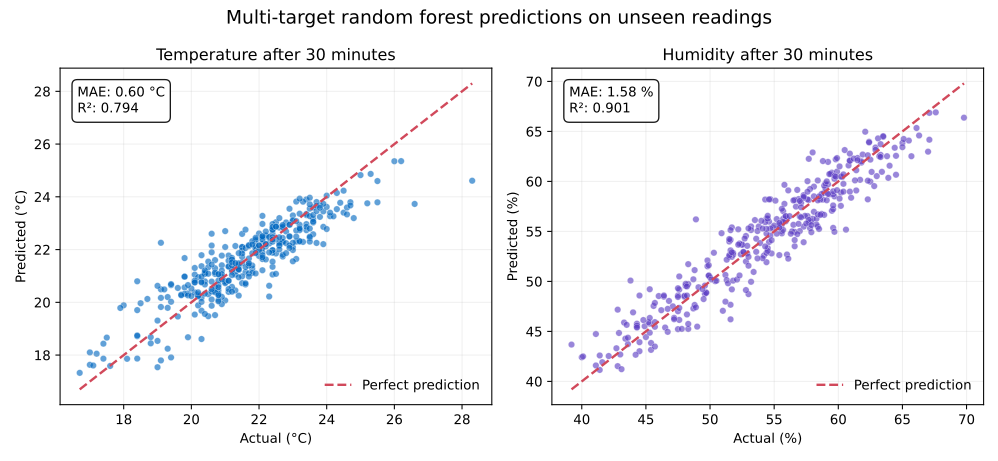
Read each panel against the dashed diagonal. A point on that line is exact. A point above it is an overprediction, and a point below it is an underprediction. The humidity points form a tighter band around the line, which agrees with humidity’s higher R².

Predict both values for a new reading

New input data must use the same feature names and units as the training data. A one-row DataFrame preserves the column names and produces a two-value prediction.

new_reading = pd.DataFrame(
    [
        {
            "outside_temp_c": 18.0,
            "solar_w_m2": 420.0,
            "inside_temp_c": 23.0,
            "inside_humidity_pct": 58.0,
            "heater_pct": 10.0,
            "vent_pct": 35.0,
            "mister_pct": 20.0,
        }
    ]
)

new_prediction = model.predict(new_reading)
named_prediction = pd.Series(
    new_prediction[0],
    index=target_columns,
).round(1)
print(named_prediction)

temp_30min_c          21.9
humidity_30min_pct    57.1
dtype: float64

For this fictional input, the model predicts 21.9 °C and 57.1% relative humidity after 30 minutes. predict() returns a two-dimensional array even for one input row, so [0] selects that row before the target names are attached.

Common mistakes and troubleshooting

Passing a one-dimensional target by accident. climate["temp_30min_c"] is a Series with shape (1800,), so it trains a single-target model. Use climate[["temp_30min_c", "humidity_30min_pct"]] or a target-column list to get shape (1800, 2).

Losing the target order. A prediction array contains values by position, not by name. Define target_columns once and use that list both when building y and when labeling predictions.

Averaging errors with different units. The default metric can average outputs into one number. That number is hard to interpret when targets use °C and percentage points. Use multioutput="raw_values", then report each result with its unit.

Using an estimator that accepts only one target. Not every regressor supports a two-dimensional y. When a suitable estimator is single-target only, MultiOutputRegressor can fit one copy of that estimator per target. The wrapper learns each target independently, while the native random forest used here builds shared tree structures for the whole target matrix.

Sending columns in a different form at prediction time. Keep the same feature names, meanings, and units. A temperature in Fahrenheit placed in a Celsius column is valid numeric input, so scikit-learn cannot detect that semantic error for you.

Reading synthetic scores as deployment evidence. The generator uses clean formulas and fixed noise. Real sensor drift, control delays, missing readings, changing seasons, and equipment faults make the task harder. Real use requires representative data, time-aware validation, safety review, and monitoring.

Skipping the output-shape check. Print predictions.shape before calculating metrics. If you expected (360, 2) and see (360,), the model trained on only one target. If you see the correct shape but swapped meanings, check target_columns.

What you learned and where to go next

Multi-target regression changes the target from one column into a matrix. The dependable workflow is:

• Build X from input columns and y from two or more named numeric target columns.
• Split features and targets together so their rows stay aligned.
• Choose an estimator with native multi-output support, such as RandomForestRegressor, or wrap a single-target estimator when needed.
• Confirm that prediction shape is (test rows, target count).
• Calculate MAE and R² separately for every target, with units and a simple baseline.
• Attach target names when showing predictions to people or sending them to another system.

The important idea is not “one model means one number.” One call to a fitted model can return a structured set of numeric answers, provided the target matrix and its column order remain clear from training through evaluation.

As a next step, add a third target such as predicted carbon-dioxide concentration. Update target_columns, rerun the same pipeline, and check whether the new target improves on its own mean baseline. For a broader view of preprocessing and model selection, continue with Preparing Data for Machine Learning.