PySpark Performance Tuning: Reading the Plan and Fixing What's Slow

You’ve got the DataFrame API down. You know select and filter are lazy, show and collect are actions, and groupBy().agg() runs in one pass over the data. Then one day a job that used to take ten seconds takes ten minutes, and none of that knowledge tells you why. The DataFrame API teaches you how to describe a computation; it doesn’t teach you how to read the computation Spark actually decided to run.

That gap is what this post closes. If you haven’t seen a Spark DataFrame before, start with PySpark for Beginners, which covers SparkSession, transformations vs. actions, and lazy evaluation from scratch. If you’re comfortable with SQL and want the query-syntax side of PySpark, Using Spark SQL in PySpark covers spark.sql(), views, and joins. This post assumes both and goes straight to the question neither one answers: your job runs, the output is correct, and it’s still too slow — now what?

The Mental Model: Performance Tuning Is Editing the Plan, Not the Code

A Spark DataFrame isn’t a table sitting in memory; it’s a recipe. Every .filter(), .join(), and .groupBy() you chain onto it adds a step to that recipe without running anything. The moment an action like .show() or .collect() finally forces execution, three things happen, in order:

1. Spark parses your recipe into a logical plan — a description of what you asked for, independent of how it will actually be computed.
2. The Catalyst optimizer rewrites that plan for cost, deciding things like join order, which join algorithm to use, and how many partitions each shuffle should produce.
3. Only then does Spark execute the rewritten plan, called the physical plan, across your machine’s cores (or a cluster’s executors).

Performance tuning almost never means rewriting your Python logic line by line. It means giving the optimizer better information, or overriding one of its defaults, so that step 2 produces a cheaper physical plan before step 3 ever touches a row. The tool for seeing what the optimizer actually decided is .explain() — call it on any DataFrame and Spark prints the physical plan it would run, without running it.

Two of the plan-level changes this post walks through, measured later on the running example below, already show what’s at stake:

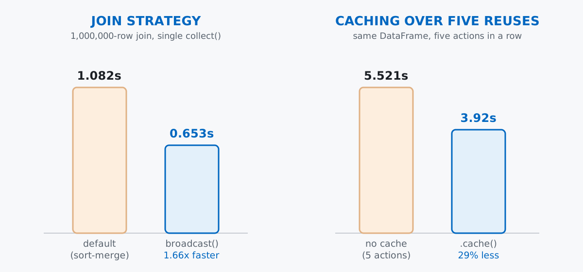
Keep that plan-first framing in mind for everything below: caching, broadcast joins, and partition counts are three different ways of handing the optimizer a cheaper plan to execute.

A Dataset You Can Reproduce: Meridian Outfitters’ Orders

Imagine a small outdoor-gear retailer, Meridian Outfitters, with a 40-item product catalog and a much larger stream of individual order lines. The catalog is exactly the shape a broadcast join is built for: small enough to fit comfortably in memory on every machine in a cluster, joined repeatedly against an orders table that’s orders of magnitude bigger.

import numpy as np
from pyspark.sql import SparkSession
from pyspark.sql import functions as F
from pyspark.sql.types import StructType, StructField, LongType, StringType, IntegerType, DoubleType

spark = (
    SparkSession.builder
    .appName("meridian-orders-perf")
    .master("local[*]")
    .getOrCreate()
)

rng = np.random.default_rng(42)

# Product catalog: 40 rows, six categories, a small lookup table
n_products = 40
categories = ["tents", "backpacks", "boots", "jackets", "cookware", "sleep-systems"]
base_price = {"tents": 180, "backpacks": 110, "boots": 95, "jackets": 140, "cookware": 45, "sleep-systems": 130}

product_rows = []
for pid in range(1, n_products + 1):
    cat = categories[(pid - 1) % len(categories)]
    price = round(float(base_price[cat] + rng.normal(0, base_price[cat] * 0.15)), 2)
    product_rows.append((pid, f"{cat}-{pid:03d}", cat, price))

products_schema = StructType([
    StructField("product_id", LongType(), False),
    StructField("product_name", StringType(), False),
    StructField("category", StringType(), False),
    StructField("unit_price", DoubleType(), False),
])
products = spark.createDataFrame(product_rows, products_schema)

# Orders: 1,000,000 rows referencing the catalog by product_id
n_orders = 1_000_000
regions = ["North America", "Europe", "APAC", "LatAm"]
region_p = [0.42, 0.31, 0.18, 0.09]

order_rows = list(zip(
    range(1, n_orders + 1),
    rng.integers(1, n_products + 1, size=n_orders).tolist(),
    rng.choice(regions, size=n_orders, p=region_p).tolist(),
    rng.integers(1, 6, size=n_orders).tolist(),
    rng.integers(0, 90, size=n_orders).tolist(),
))
orders_schema = StructType([
    StructField("order_id", LongType(), False),
    StructField("product_id", LongType(), False),
    StructField("region", StringType(), False),
    StructField("quantity", IntegerType(), False),
    StructField("day_offset", IntegerType(), False),
])
orders = spark.createDataFrame(order_rows, orders_schema)

print(products.count(), orders.count())

40 1000000

Forty products, a million order lines. (The outputs in this post come from PySpark 3.5.3 on Python 3.11 — the same pinned version used in the two prerequisite posts, since a plain pip install pyspark currently grabs 4.x, which needs a newer JDK than this machine has.) A million rows is tiny by Spark’s real-world standards, but it’s enough for the gap between a good plan and a bad one to show up in real seconds on a single laptop.

Reading a Real .explain() Plan

Start with a query that joins orders to products and totals revenue per region:

region_totals = (
    orders
    .join(products, "product_id")
    .withColumn("line_total", F.col("quantity") * F.col("unit_price"))
    .groupBy("region")
    .agg(F.round(F.sum("line_total"), 2).alias("total_revenue"))
    .orderBy("region")
)
region_totals.explain()

== Physical Plan ==
AdaptiveSparkPlan isFinalPlan=false
+- Sort [region#36 ASC NULLS FIRST], true, 0
   +- Exchange rangepartitioning(region#36 ASC NULLS FIRST, 200), ENSURE_REQUIREMENTS, [plan_id=135]
      +- HashAggregate(keys=[region#36], functions=[sum(line_total#83)])
         +- Exchange hashpartitioning(region#36, 200), ENSURE_REQUIREMENTS, [plan_id=132]
            +- HashAggregate(keys=[region#36], functions=[partial_sum(line_total#83)])
               +- Project [region#36, (cast(quantity#37 as double) * unit_price#3) AS line_total#83]
                  +- SortMergeJoin [product_id#35L], [product_id#0L], Inner
                     :- Sort [product_id#35L ASC NULLS FIRST], false, 0
                     :  +- Exchange hashpartitioning(product_id#35L, 200), ENSURE_REQUIREMENTS, [plan_id=124]
                     :     +- Project [product_id#35L, region#36, quantity#37]
                     :        +- Scan ExistingRDD[order_id#34L,product_id#35L,region#36,quantity#37,day_offset#38]
                     +- Sort [product_id#0L ASC NULLS FIRST], false, 0
                        +- Exchange hashpartitioning(product_id#0L, 200), ENSURE_REQUIREMENTS, [plan_id=125]
                           +- Project [product_id#0L, unit_price#3]
                              +- Scan ExistingRDD[product_id#0L,product_name#1,category#2,unit_price#3]

Read it from the bottom up — that’s the order data actually flows in. Each Scan ExistingRDD is a source reading in. Every Exchange is a shuffle: Spark redistributes rows across partitions — over the network on a real cluster, across cores here — so rows that need to be together (matching join keys, matching group keys) land in the same partition. This plan has four: one shuffle per side of the SortMergeJoin to sort both sides by product_id, a third to regroup by region for the aggregation, and a fourth to range-partition for the final orderBy. Shuffles are expensive because they write data to disk, move it across partitions, and read it back — the single biggest cost in most slow Spark jobs is shuffles you didn’t know you were paying for.

Notice the 200 inside hashpartitioning(product_id#35L, 200) — that’s spark.sql.shuffle.partitions, the number of partitions Spark uses for any shuffle, completely independent of how many partitions your source DataFrame actually has. It defaults to 200, a number from an era when Spark clusters routinely had hundreds of cores; on a 10-core laptop it means a shuffle here fans out into 200 small partitions that then have to be scheduled back down onto 10 cores. Keep this in mind — it resurfaces in the partitioning section below.

You don’t need to parse every line of a plan like this to use it. The two questions worth asking first are: how many Exchange nodes are there, and which join algorithm is being used (SortMergeJoin here — a broadcast join, covered next, shows up as BroadcastHashJoin instead and skips one of those shuffles entirely).

Caching a Reused DataFrame with .cache()

region_totals above is used once. But it’s common to build one enriched DataFrame and then run several different summaries against it — exactly the case where Spark’s laziness works against you, because every action re-runs the entire upstream plan from scratch, including the join, by default:

def build_enriched(src_orders, src_products):
    return (
        src_orders
        .join(src_products, "product_id")
        .withColumn("line_total", F.round(F.col("quantity") * F.col("unit_price"), 2))
        .withColumn("is_bulk", F.col("quantity") >= 4)
        .filter(F.col("unit_price") > 40)
    )

enriched = build_enriched(orders, products)

import time

def timed(label, fn):
    t0 = time.perf_counter()
    result = fn()
    dt = time.perf_counter() - t0
    print(f"{label}: {result} ({dt:.3f}s)")
    return dt

t_count = timed("count", lambda: enriched.count())
t_avg = timed("avg_line_total", lambda: enriched.agg(F.round(F.avg("line_total"), 2).alias("x")).collect()[0]["x"])
t_bulk = timed("bulk_count", lambda: enriched.filter(F.col("is_bulk")).count())
t_max = timed("max_line_total", lambda: enriched.agg(F.max("line_total").alias("x")).collect()[0]["x"])
t_cat = timed("category_counts", lambda: len(enriched.groupBy("category").count().collect()))

print("no_cache_total:", round(t_count + t_avg + t_bulk + t_max + t_cat, 3))

count: 974568 (1.419s)
avg_line_total: 363.77 (1.355s)
bulk_count: 390242 (0.783s)
max_line_total: 1189.1 (0.99s)
category_counts: 6 (0.974s)
no_cache_total: 5.521

Five actions, and the join-plus-filter reruns five times — 5.52 seconds total. Now cache it:

enriched_cached = build_enriched(orders, products).cache()

t_count = timed("count", lambda: enriched_cached.count())            # materializes the cache
t_avg = timed("avg_line_total", lambda: enriched_cached.agg(F.round(F.avg("line_total"), 2).alias("x")).collect()[0]["x"])
t_bulk = timed("bulk_count", lambda: enriched_cached.filter(F.col("is_bulk")).count())
t_max = timed("max_line_total", lambda: enriched_cached.agg(F.max("line_total").alias("x")).collect()[0]["x"])
t_cat = timed("category_counts", lambda: len(enriched_cached.groupBy("category").count().collect()))

print("with_cache_total:", round(t_count + t_avg + t_bulk + t_max + t_cat, 3))

count: 974568 (2.646s)
avg_line_total: 363.77 (0.35s)
bulk_count: 390242 (0.275s)
max_line_total: 1189.1 (0.245s)
category_counts: 6 (0.404s)
with_cache_total: 3.92

Look at the first action, count: it’s slower cached (2.646s) than uncached (1.419s), because .cache() doesn’t load anything by itself — it’s still lazy — and the first action that touches enriched_cached has to run the full plan and write the result into memory. That’s the cost of caching. But every action after that drops to a fraction of a second, because it now reads from memory instead of re-running the join. By the third action, the cached version has already overtaken the uncached total (3.271s cached vs. 3.557s uncached, cumulatively), and by the fifth it’s 3.92s against 5.521s — roughly 29% less total time for the same five summaries. .persist() is the same idea with a chosen storage level (.cache() is shorthand for .persist(StorageLevel.MEMORY_AND_DISK)); reach for it when you need to spill to disk instead of dropping cached partitions that don’t fit in memory.

The takeaway isn’t “always cache” — it’s “cache pays for itself only after enough reuse.” One or two actions against a DataFrame, and the write-to-cache overhead alone can make you slower, not faster.

Broadcast Joins for a Small Lookup Table

The SortMergeJoin from the .explain() section shuffles both sides of the join across the network or across cores. That’s wasteful when one side, like our 40-row product catalog, is small enough to just hand a full copy to every partition instead. That’s a broadcast join: skip shuffling the small table entirely, and let each partition of the large table look up matches locally.

Spark’s optimizer can do this automatically for tables under spark.sql.autoBroadcastJoinThreshold (10 MB by default), but automatic size estimation doesn’t always kick in — DataFrames built directly from in-memory Python data, like ours, don’t carry the file-based size statistics the optimizer relies on. Turn the threshold off entirely to force a plain shuffle join and get an honest “before” measurement:

spark.conf.set("spark.sql.autoBroadcastJoinThreshold", -1)

default_join = orders.join(products, "product_id").groupBy("region").agg(F.sum("quantity").alias("units"))

t0 = time.perf_counter()
default_join.orderBy("region").collect()
default_join_time = time.perf_counter() - t0
print("default_join_time:", round(default_join_time, 3))

default_join_time: 1.082

Now hint the join explicitly with F.broadcast():

from pyspark.sql import functions as F

broadcast_join = orders.join(F.broadcast(products), "product_id").groupBy("region").agg(F.sum("quantity").alias("units"))
broadcast_join.explain()

t0 = time.perf_counter()
broadcast_join.orderBy("region").collect()
broadcast_join_time = time.perf_counter() - t0
print("broadcast_join_time:", round(broadcast_join_time, 3))
print("speedup:", round(default_join_time / broadcast_join_time, 2))

== Physical Plan ==
AdaptiveSparkPlan isFinalPlan=false
+- HashAggregate(keys=[region#36], functions=[sum(quantity#37)])
   +- Exchange hashpartitioning(region#36, 200), ENSURE_REQUIREMENTS, [plan_id=1773]
      +- HashAggregate(keys=[region#36], functions=[partial_sum(quantity#37)])
         +- Project [region#36, quantity#37]
            +- BroadcastHashJoin [product_id#35L], [product_id#0L], Inner, BuildRight, false
               :- Project [product_id#35L, region#36, quantity#37]
               :  +- Scan ExistingRDD[order_id#34L,product_id#35L,region#36,quantity#37,day_offset#38]
               +- BroadcastExchange HashedRelationBroadcastMode(List(input[0, bigint, false]),false), [plan_id=1768]
                  +- Project [product_id#0L]
                     +- Scan ExistingRDD[product_id#0L,product_name#1,category#2,unit_price#3]

broadcast_join_time: 0.653
speedup: 1.66

The SortMergeJoin is gone, replaced by BroadcastHashJoin with a BroadcastExchange on the small side only — the large orders table is no longer shuffled at all. On this run that’s a 1.66x speedup on the join itself; the gap widens further on a real cluster, where the shuffle side of a sort-merge join also crosses the network between machines, not just cores on one laptop. For details on when Spark applies this automatically and how to tune the threshold, see Spark’s SQL performance tuning guide, which documents autoBroadcastJoinThreshold and the other join-related settings this post doesn’t cover.

Partition Count and Parallelism: .repartition() and .coalesce()

A DataFrame’s rows are split across partitions, and Spark processes one task per partition, in parallel, up to however many cores you have. Too few partitions and you leave cores idle; too many and the overhead of scheduling each tiny task starts to dominate the actual work. .repartition(n) reshuffles into exactly n partitions (useful to increase parallelism); .coalesce(n) merges partitions down to n without a full shuffle (useful to decrease it cheaply, e.g. before writing out fewer output files).

print("orders.rdd.getNumPartitions():", orders.rdd.getNumPartitions())

one_partition = orders.coalesce(1)
t0 = time.perf_counter()
one_partition.groupBy("region").agg(F.sum("quantity").alias("units")).collect()
too_few_time = time.perf_counter() - t0

t0 = time.perf_counter()
orders.groupBy("region").agg(F.sum("quantity").alias("units")).collect()
default_time = time.perf_counter() - t0

many_partitions = orders.repartition(400)
t0 = time.perf_counter()
many_partitions.groupBy("region").agg(F.sum("quantity").alias("units")).collect()
too_many_time = time.perf_counter() - t0

print("too_few (1 partition):", round(too_few_time, 3))
print("default (10 partitions):", round(default_time, 3))
print("too_many (400 partitions):", round(too_many_time, 3))

orders.rdd.getNumPartitions(): 10
too_few (1 partition): 1.285
default (10 partitions): 0.466
too_many (400 partitions): 1.757

This machine has 10 CPU cores, and orders already sits at 10 partitions by default — one task per core, nothing idle, nothing oversplit. Collapsing to a single partition with .coalesce(1) forces every row through one task, so nine cores sit idle: 1.285 seconds, nearly three times slower. Going the other way with .repartition(400) is worse still, at 1.757 seconds — the actual aggregation work hasn’t grown, but Spark now has to schedule, serialize, and collect results from 400 separate tasks instead of 10, and that bookkeeping costs more than the extra parallelism buys back on a dataset this size. The right partition count isn’t a fixed number; it’s “enough to use your cores (or executors) without creating more tasks than there’s work to justify.”

Four Gotchas Worth Knowing

Caching everything “just in case” costs more than it saves. The measurement above showed it directly: the first action against a freshly cached DataFrame was slower than the same action with no cache at all (2.646s vs. 1.419s), because writing the result into memory is extra work on top of computing it. If a DataFrame gets touched once or twice, don’t cache it — you’ll pay the write cost and never earn it back.

A broadcast join can blow up memory if the “small” table stops being small. spark.sql.autoBroadcastJoinThreshold exists precisely to stop Spark from auto-broadcasting a table that’s grown past a safe size. An explicit F.broadcast() hint bypasses that safety check entirely — you’re telling Spark to ship a full copy of that table to every executor no matter how big it’s gotten. A 40-row product catalog is safe. The same code left in place after the catalog grows to four million SKUs will try to broadcast gigabytes to every executor and can crash the job with an out-of-memory error instead of just running slowly.

Too many small partitions add scheduling overhead that outweighs the parallelism they’re supposed to buy. The 400-partition run above wasn’t a pathological case — it’s what .repartition() with an arbitrarily large number does on any dataset that doesn’t need that much parallelism. Each partition still needs its own task, and task scheduling isn’t free.

.explain() output looks intimidating, but you only need the top-level shape at first. Read it bottom to top, count the Exchange nodes (each one is a shuffle), and note the join algorithm. You don’t need to parse every #83-style column reference to get useful signal from a plan.

Wrapping Up

Every tool in this post does the same thing from a different angle: give Spark’s optimizer a cheaper plan before execution starts.

• .explain() — read the physical plan; count Exchange nodes to count shuffles, and check the join algorithm
• .cache() / .persist() — pay once to materialize a DataFrame you’ll reuse three or more times; skip it for one-off DataFrames
• F.broadcast() — skip shuffling the large side of a join when the other side is genuinely small, but never on a table whose size you can’t guarantee
• .repartition() / .coalesce() — match partition count to available cores or executors, not to a round number

If you want the SQL-shaped side of PySpark — registering views, writing spark.sql() queries, and joins — Using Spark SQL in PySpark picks up right where this post’s .explain() section leaves off, since every spark.sql() query compiles to the same kind of physical plan shown above. And if any of the DataFrame calls in this post looked unfamiliar, PySpark for Beginners covers the API these tuning techniques sit on top of. One thing worth saying plainly: none of this matters if your data comfortably fits in memory on a single machine — the Pandas Data Analysis lessons in our free Python for Data Analytics course cover the same joins, groupings, and aggregations without ever paying Spark’s distributed-execution overhead in the first place.