How many bicycles will people rent during the next hour? Will the station be nearly empty by the end of that hour? These questions start from the same station data, but one answer is a number and the other is a class.

To build a multi-task PyTorch model for regression and binary classification, pass the inputs through shared layers and connect that shared representation to two output heads. Train the numeric head with a regression loss, train the class head with a classification loss, combine the losses before backpropagation, and measure each output with task-specific test metrics.

This lesson implements that pattern for a fictional bike-share station. The model predicts the next-hour rental count and the chance that no more than three bicycles will remain. The focus is the structure of a mixed-output model, not transport planning.

Setup and the synthetic station data

You need Python 3.11 or newer and basic experience with Python functions and pandas tables. You should also know that a train set teaches a model and a test set checks it on unseen rows. If that split is new to you, begin with How to Build Your First Machine Learning Model.

Create a virtual environment if you want an isolated package set. Then install the libraries used by the executed lesson:

python -m venv .venv
source .venv/bin/activate
python -m pip install numpy pandas scikit-learn torch matplotlib

On Windows PowerShell, activate the environment with .venv\Scripts\Activate.ps1. The results below used Python 3.13.2, NumPy 2.5.1, pandas 3.0.3, scikit-learn 1.9.0, PyTorch 2.12.0, and Matplotlib 3.11.0 on a CPU.

Download bike_station_hours.csv and place it beside your Python file. It contains 2,400 original synthetic rows generated with NumPy seed 73. Synthetic means that code created the data. The stations, weather, inventory, rentals, and labels are fictional and released under CC0-1.0.

Load the table and inspect only three rows. A small preview makes both targets and their units clear before tensors hide the column names:

import pandas as pd

station_hours = pd.read_csv("bike_station_hours.csv")

print(station_hours.shape)
print(station_hours.head(3).to_string(index=False))
print(station_hours["empty_next_hour"].value_counts().sort_index())

(2400, 12)
station_hour_id  hour  hour_sin  hour_cos  temperature_c  rain_mm  weekend  nearby_event  bikes_available  empty_docks  next_hour_rentals  empty_next_hour
        BS-0001    19  -0.96593   0.25882           14.5      3.1        0             0               23           17                 13                0
        BS-0002    11   0.25882  -0.96593           24.7      3.4        1             0               15           25                 20                0
        BS-0003    18  -1.00000  -0.00000           11.9      0.0        1             0                9           31                 11                0
empty_next_hour
0    1982
1     418
Name: count, dtype: int64

next_hour_rentals is the regression target. Regression predicts a numeric value. empty_next_hour is the binary classification target: 1 means that three or fewer bicycles remain, and 0 means more remain.

The class is imbalanced because only 17.4% of rows have label 1. Later, accuracy alone will not be enough to judge this head. The identifier is not a model feature, and the raw hour column is also excluded. Its cyclic versions, hour_sin and hour_cos, place hour 23 close to hour 0.

How one shared trunk works with two heads

Multi-task learning trains one model on several related prediction tasks. Our model has three parts:

8 station features
        |
 shared layers
   /         \
rental head  empty-station head
one number   one raw class score

The shared layers are often called the trunk. They can learn patterns useful to both tasks, such as how commuting hours, rain, and current inventory interact. A head is the final task-specific part. One head may need a different output shape and loss from another.

For a batch of 64 rows, the shapes are:

input features:       (64, 8)
rental prediction:    (64, 1)
empty-station logit:  (64, 1)

A logit is a raw classification score before conversion to a probability. It can be any real number. torch.sigmoid() changes it to a value from 0 to 1 when we need an estimated probability.

This structure does not force the two predictions to agree. It only lets them learn a shared internal representation. A poor match between the tasks can even make joint training worse. You still need separate validation and test evidence for both outputs.

PyTorch models inherit from nn.Module. Its current module guidance allows forward() to perform arbitrary computation with any number of inputs and outputs. We use that flexibility to return a tuple:

import torch
from torch import nn


class StationMultiTaskNet(nn.Module):
    def __init__(self, input_features):
        super().__init__()
        self.shared = nn.Sequential(
            nn.Linear(input_features, 32),
            nn.ReLU(),
            nn.Linear(32, 16),
            nn.ReLU(),
        )
        self.rental_head = nn.Linear(16, 1)
        self.empty_head = nn.Linear(16, 1)

    def forward(self, features):
        shared_features = self.shared(features)
        rental_prediction = self.rental_head(shared_features)
        empty_logit = self.empty_head(shared_features)
        return rental_prediction, empty_logit

Both heads receive the same 16 shared values. They do not receive each other’s prediction. That detail matters: the class head can learn from shared features, but it is not a rule that labels a row from the predicted rental count.

Keep all three data groups aligned

Training needs three groups. Training rows update weights, validation rows select a checkpoint, and test rows provide one final check.

Name the eight input columns explicitly. Then split the complete table twice. stratify keeps the rare empty-station rate close to 17.4% in every group:

from sklearn.model_selection import train_test_split

feature_columns = [
    "hour_sin",
    "hour_cos",
    "temperature_c",
    "rain_mm",
    "weekend",
    "nearby_event",
    "bikes_available",
    "empty_docks",
]

development, test = train_test_split(
    station_hours,
    test_size=0.20,
    random_state=73,
    stratify=station_hours["empty_next_hour"],
)
train, validation = train_test_split(
    development,
    test_size=0.20,
    random_state=73,
    stratify=development["empty_next_hour"],
)

for name, frame in [
    ("train", train),
    ("validation", validation),
    ("test", test),
]:
    print(name, len(frame), round(frame["empty_next_hour"].mean(), 3))

train 1536 0.174
validation 384 0.174
test 480 0.175

Each split operation moves whole rows, so the features and both targets cannot drift out of alignment.

Neural networks learn more easily when numeric columns have similar scales. Fit a StandardScaler on training features only. Its official reference explains that it stores the training mean and standard deviation for later calls to transform().

We also standardize the rental target. This is not required for every regression network, but it gives our regression loss a manageable scale before we add it to the classification loss. A rental value is changed to the number of training standard deviations above or below the training mean.

from sklearn.preprocessing import StandardScaler

feature_scaler = StandardScaler()
rental_scaler = StandardScaler()

X_train = feature_scaler.fit_transform(train[feature_columns])
X_validation = feature_scaler.transform(validation[feature_columns])
X_test = feature_scaler.transform(test[feature_columns])

y_rental_train = rental_scaler.fit_transform(
    train[["next_hour_rentals"]]
)
y_rental_validation = rental_scaler.transform(
    validation[["next_hour_rentals"]]
)

Do not call fit_transform() on validation or test data. That would let their averages influence model preparation. It would also give each group a different coordinate system.

Now convert the arrays to 32-bit floating-point tensors. Keep both targets shaped (rows, 1) so they match their output heads:

def as_float_tensor(values):
    return torch.tensor(values, dtype=torch.float32)


X_train = as_float_tensor(X_train)
X_validation = as_float_tensor(X_validation)
X_test = as_float_tensor(X_test)

y_rental_train = as_float_tensor(y_rental_train)
y_rental_validation = as_float_tensor(y_rental_validation)
y_empty_train = as_float_tensor(
    train[["empty_next_hour"]].to_numpy()
)
y_empty_validation = as_float_tensor(
    validation[["empty_next_hour"]].to_numpy()
)

print(X_train.shape)
print(y_rental_train.shape)
print(y_empty_train.shape)

torch.Size([1536, 8])
torch.Size([1536, 1])
torch.Size([1536, 1])

Train both tasks with one backward pass

A DataLoader groups rows into batches. PyTorch’s data-loading documentation states that automatic batching adds the batch dimension and preserves tuple structure. Our tuple contains features, a rental target, and an empty-station target:

from torch.utils.data import DataLoader, TensorDataset

train_data = TensorDataset(
    X_train,
    y_rental_train,
    y_empty_train,
)
loader_generator = torch.Generator().manual_seed(73)
train_loader = DataLoader(
    train_data,
    batch_size=64,
    shuffle=True,
    generator=loader_generator,
    num_workers=0,
)

Create the model and one loss function per head. SmoothL1Loss behaves quadratically for small regression errors and linearly for larger ones. The PyTorch reference describes it as less sensitive to outliers than mean squared error.

BCEWithLogitsLoss handles binary classification. It combines the sigmoid calculation and binary cross-entropy in a numerically stable operation. For this reason, the class head returns a logit rather than applying sigmoid inside forward().

model = StationMultiTaskNet(input_features=len(feature_columns))
optimizer = torch.optim.Adam(model.parameters(), lr=0.002)

rental_loss_function = nn.SmoothL1Loss(beta=0.5)
empty_loss_function = nn.BCEWithLogitsLoss()

The next loop shows the central multi-task step for one epoch. It calculates two losses, adds them, and calls backward() once. Gradients from both losses reach the shared layers. Each head also receives gradients from its own loss:

model.train()

for feature_batch, rental_batch, empty_batch in train_loader:
    predicted_rentals, empty_logits = model(feature_batch)

    rental_loss = rental_loss_function(
        predicted_rentals,
        rental_batch,
    )
    empty_loss = empty_loss_function(
        empty_logits,
        empty_batch,
    )
    total_loss = rental_loss + empty_loss

    optimizer.zero_grad()
    total_loss.backward()
    optimizer.step()

The equal addition is a starting choice, not a universal rule. It is reasonable here because the rental target was standardized and both loss functions return batch means. Always print or record the individual losses. If one remains 100 times larger, it may control nearly every shared-layer update.

The executed build repeats that batch loop for up to 300 epochs. After each epoch, it measures both validation losses without updating weights. It saves a checkpoint when their sum improves by at least 0.0001, then stops after 30 epochs without an improvement of that size:

import copy

best_validation_loss = float("inf")
best_model_state = None

# Inside the epoch loop, after measuring validation losses:
validation_total = validation_rental_loss + validation_empty_loss

if validation_total < best_validation_loss - 0.0001:
    best_validation_loss = validation_total
    best_model_state = copy.deepcopy(model.state_dict())

# After early stopping:
model.load_state_dict(best_model_state)

The run stopped after 79 epochs and restored epoch 49:

best epoch: 49 of 79

The fixed NumPy, PyTorch, split, and loader seeds make this lesson repeatable in its tested environment. PyTorch’s reproducibility notes warn that exact results are not guaranteed across releases, platforms, or CPU and GPU execution.

Evaluate each task with its own metrics

The rental head predicts standardized values, so convert them back to rental counts. The class head still returns logits, so apply sigmoid and use 0.5 as the label threshold:

model.eval()

with torch.no_grad():
    rental_scaled, empty_logits = model(X_test)
    empty_probability = torch.sigmoid(empty_logits).numpy().ravel()

rental_prediction = rental_scaler.inverse_transform(
    rental_scaled.numpy()
).ravel()
empty_prediction = (empty_probability >= 0.5).astype(int)

model.eval() switches layers that behave differently during training to evaluation mode. This small network does not use dropout or batch normalization, but the call keeps the prediction code correct if such layers are added later. torch.no_grad() avoids building a gradient graph because evaluation does not update weights.

Four test rows make the two outputs concrete:

      actual_rentals  predicted_rentals  actual_empty  empty_probability  predicted_empty
247               24             25.161             1              0.706                1
757               16             20.914             0              0.039                0
505               15             19.273             0              0.665                1
1260               7              4.714             0              0.000                0

Row 247 is close on both tasks: its rental prediction is about 1.2 above the actual count, and its empty-station class is correct. Row 505 is a false alarm because its empty probability is above 0.5 while the actual class is 0.

Mean absolute error, or MAE, measures the average absolute rental-count error. For the class head, precision measures how many predicted empty cases were empty. Recall measures how many actual empty cases the model found. F1 combines precision and recall into one balance:

rental MAE: 3.108
rental median baseline MAE: 7.660
empty metrics: accuracy=0.906 precision=0.791 recall=0.631 f1=0.702
empty majority baseline accuracy: 0.825
confusion matrix:
[[382  14]
 [ 31  53]]

The rental head misses by 3.11 rentals on average and beats the training-median baseline at 7.66. The class head correctly labels 90.6% of test rows, compared with 82.5% from always predicting the majority class.

The confusion matrix adds an important limit. The model finds 53 of 84 empty cases, which gives 0.631 recall, but misses 31. A real station operator might prefer a lower threshold to find more empty cases, even if that produces more false alarms. That decision needs operational costs and representative real data.

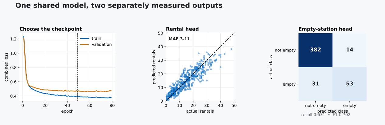
Read the center panel against its dashed diagonal. Points on the line are exact rental predictions; vertical distance from the line is error. In the right panel, rows are actual classes and columns are predicted classes. The lower-left count of 31 is the missed-empty group that accuracy alone hides.

Make both predictions for one new hour

New rows must use the same eight feature meanings, column order, and units. The example describes 17:00 on a weekday, with an event nearby, no rain, and 12 bicycles available:

import numpy as np

new_hour = pd.DataFrame(
    [{
        "hour_sin": np.sin(2 * np.pi * 17 / 24),
        "hour_cos": np.cos(2 * np.pi * 17 / 24),
        "temperature_c": 21.0,
        "rain_mm": 0.0,
        "weekend": 0,
        "nearby_event": 1,
        "bikes_available": 12,
        "empty_docks": 28,
    }]
)

new_features = as_float_tensor(
    feature_scaler.transform(new_hour)
)

model.eval()
with torch.no_grad():
    rental_scaled, empty_logit = model(new_features)

predicted_rentals = rental_scaler.inverse_transform(
    rental_scaled.numpy()
)[0, 0]
empty_probability = torch.sigmoid(empty_logit).item()

print(f"predicted rentals: {predicted_rentals:.1f}")
print(f"empty probability: {empty_probability:.3f}")
print(f"predicted class: {int(empty_probability >= 0.5)}")

predicted rentals: 39.3
empty probability: 0.854
predicted class: 1

The model returns both answers in one call: about 39 rentals and class 1. Do not treat 0.854 as a verified real-world probability. Probability calibration was not tested, and the complete dataset is synthetic.

Common mistakes and troubleshooting

Applying sigmoid twice. Pass raw logits from the class head to BCEWithLogitsLoss. Apply sigmoid only when you need probabilities. A sigmoid layer inside the model followed by BCEWithLogitsLoss repeats the transformation.

Using different shapes for logits and class targets. This lesson keeps both at (batch, 1). The BCEWithLogitsLoss documentation requires input and target to have the same shape. Do not remove only one singleton dimension.

Adding incomparable losses without inspection. A regression loss on raw values may be much larger than a classification loss. Standardize the numeric target or set documented task weights, then record each loss separately. Equal weights do not mean equal influence automatically.

Fitting scalers before the split. That leaks validation and test statistics into preparation. Split complete rows first. Fit feature and target scalers on training rows only, then reuse them everywhere.

Converting scaled predictions directly to counts. The rental head learned standardized targets. Call rental_scaler.inverse_transform() before calculating rental-count MAE or showing a prediction.

Judging both heads with one score. Combined loss is useful for training and checkpoint selection, but it does not explain final behavior. Report rental error in rentals and class errors with a confusion matrix, precision, and recall.

Treating a shared trunk as guaranteed improvement. Related tasks can support each other, but they can also compete. Compare with credible single-task models on the same splits before choosing multi-task learning for a real system.

Reading synthetic results as transport evidence. The generator omits station closures, broken bicycles, data delays, holidays, changing routes, and unusual demand. A deployed model needs representative history, time-aware validation, probability checks, monitoring, and human review.

Recap: share features, not evaluation

A mixed-output model can return a number and a class from one input row. The shared trunk learns reusable features, while separate heads keep the output shapes and meanings distinct.

The dependable workflow is to split complete rows, fit preprocessing on training data, standardize a large-scale numeric target when needed, and match each head with its own loss. Add the losses for one backward pass, but keep their values visible and validate the chosen weighting.

The final rule is simple: share the representation, not the evaluation. This run selected epoch 49, reached a rental MAE of 3.11, and found 53 of 84 empty-station cases. Those results answer different questions, so neither should disappear inside one combined score.

As a next experiment, test classification thresholds from 0.2 to 0.8 without retraining the model. Plot recall and false alarms at each threshold, then choose a threshold only after stating which error matters more for the intended use.