Build a Reproducible Machine Learning Snapshot with SQLite

A model can be reproducible while its training data is not. You may save the random seed and model settings, then rerun the project a week later and get different results because the source table has gained new rows.

This tutorial fixes that problem before model training begins. We will turn hourly greenhouse sensor readings into one daily feature row per zone. Every build records a cutoff, which is the latest time a source reading may have. Rows that arrive later cannot silently change an existing snapshot.

The result is a small feature snapshot: a stored table of model inputs linked to a recorded build run. We use SQLite because it is included with Python and stores the whole database in one local file. The same design also works in larger database systems.

Prerequisites and setup

You need Python 3.10 or newer. You should be comfortable running a Python script, but you do not need previous machine learning or database experience.

The data work uses Python’s built-in csv and sqlite3 modules. Matplotlib creates the final data-quality chart:

python3 -m venv .venv
source .venv/bin/activate
python -m pip install matplotlib==3.11.0

On Windows PowerShell, activate with .venv\Scripts\Activate.ps1. The published results were tested with Python 3.13.2, SQLite 3.50.2, and Matplotlib 3.11.0.

Download the tutorial’s synthetic greenhouse readings and save the CSV in the same folder as your script. It contains 714 fictional readings from three greenhouse zones over ten days. The dataset was generated deterministically for this lesson and is released under the CC0 1.0 public-domain dedication.

The mental model: three data layers

We will keep three kinds of data separate:

1. Raw readings record what each sensor reported and when.
2. Run metadata records how and when a snapshot was defined.
3. Features contain the numeric inputs that a model can use.

A feature is a value prepared for a model. For example, one temperature reading is raw data. The average temperature for a zone on one day is a feature.

The separation matters. Raw data may continue growing, while a finished feature snapshot must keep the same meaning. A run_id connects every feature row to its cutoff and feature definition.

For this lesson, the cutoff is 2026-06-08 00:00:00. Only measurements before that moment may enter run 1. The CSV also contains readings from June 8 through June 10, so we can verify that the filter works.

Create tables that reject invalid data

Open a database connection and enable foreign-key checks. A foreign key is a rule that requires a value to point to an existing row in another table.

import sqlite3

connection = sqlite3.connect("greenhouse_features.db")
connection.execute("PRAGMA foreign_keys = ON")

Next, create the three tables. Read the constraints as data-quality rules: a zone must be known, humidity must be between 0 and 100, and a zone cannot report twice at the same time.

connection.executescript("""
CREATE TABLE sensor_readings (
    reading_id INTEGER PRIMARY KEY,
    zone TEXT NOT NULL CHECK (zone IN ('north', 'central', 'south')),
    measured_at TEXT NOT NULL,
    temperature_c REAL NOT NULL CHECK (temperature_c BETWEEN -20 AND 60),
    humidity_pct REAL NOT NULL CHECK (humidity_pct BETWEEN 0 AND 100),
    UNIQUE (zone, measured_at)
) STRICT;

CREATE TABLE feature_runs (
    run_id INTEGER PRIMARY KEY,
    cutoff_at TEXT NOT NULL,
    feature_definition TEXT NOT NULL,
    created_at TEXT NOT NULL
) STRICT;

CREATE TABLE daily_features (
    run_id INTEGER NOT NULL REFERENCES feature_runs(run_id),
    zone TEXT NOT NULL,
    feature_date TEXT NOT NULL,
    reading_count INTEGER NOT NULL,
    mean_temperature_c REAL NOT NULL,
    temperature_range_c REAL NOT NULL,
    mean_humidity_pct REAL NOT NULL,
    PRIMARY KEY (run_id, zone, feature_date)
) STRICT;
""")

STRICT asks SQLite to enforce the declared storage types. CHECK, NOT NULL, and UNIQUE add rules that types alone cannot express. SQLite’s official STRICT tables guide explains the supported types and how strict tables interact with integrity checks.

These rules fail early. A humidity value of 140 raises an error during loading instead of reaching model training as a hard-to-find outlier.

Load the CSV with parameters and one transaction

CSV values start as text, so convert numeric fields explicitly. This small transformation also makes the expected schema visible in the code.

import csv

with open("greenhouse_sensor_readings.csv", newline="", encoding="utf-8") as handle:
    rows = [
        (
            int(row["reading_id"]),
            row["zone"],
            row["measured_at"],
            float(row["temperature_c"]),
            float(row["humidity_pct"]),
        )
        for row in csv.DictReader(handle)
    ]

Now insert those tuples. The five ? characters are placeholders. The database driver binds each value separately from the SQL statement.

with connection:
    connection.executemany(
        "INSERT INTO sensor_readings VALUES (?, ?, ?, ?, ?)",
        rows,
    )

raw_count = connection.execute(
    "SELECT COUNT(*) FROM sensor_readings"
).fetchone()[0]
print("raw rows:", raw_count)

raw rows: 714

The with connection: block is a transaction boundary. A transaction treats a group of database changes as one unit: SQLite commits all inserts when the block finishes successfully, or rolls them back if an error occurs. The block does not close the connection.

Do not replace placeholders with an f-string. Parameter binding handles quoting safely and prevents input from being interpreted as SQL. Python’s official sqlite3 guide documents both question-mark and named placeholders.

Record the run before building features

The feature calculation needs a durable identity. Insert one row into feature_runs before inserting the feature rows:

CUTOFF = "2026-06-08 00:00:00"

with connection:
    cursor = connection.execute(
        """
        INSERT INTO feature_runs (cutoff_at, feature_definition, created_at)
        VALUES (?, ?, ?)
        """,
        (
            CUTOFF,
            "daily zone aggregates v1: count, mean/range temperature, mean humidity",
            "2026-07-14 12:00:00",
        ),
    )
    run_id = cursor.lastrowid

print("run id:", run_id)

run id: 1

In a production pipeline, created_at would usually come from a clock in Coordinated Universal Time (UTC). We use a fixed value here so every learner gets identical artifacts. The important fields are the cutoff and the feature definition. Together, they answer: Which source rows and which calculation produced this snapshot?

Build the snapshot with one SQL statement

The next query selects only eligible readings, groups them by zone and calendar date, and calculates four features. INSERT INTO ... SELECT writes the query result directly into the feature table.

with connection:
    connection.execute(
        """
        INSERT INTO daily_features
        SELECT
            ?,
            zone,
            date(measured_at),
            COUNT(*),
            ROUND(AVG(temperature_c), 2),
            ROUND(MAX(temperature_c) - MIN(temperature_c), 2),
            ROUND(AVG(humidity_pct), 2)
        FROM sensor_readings
        WHERE measured_at < ?
        GROUP BY zone, date(measured_at)
        """,
        (run_id, CUTOFF),
    )

The order is important. WHERE removes readings at or after the cutoff. GROUP BY then creates one group per zone and date. Aggregate functions such as AVG and MAX turn each group into one feature row.

Inspect a few rows rather than trusting a successful query:

sample = connection.execute(
    """
    SELECT feature_date, zone, reading_count, mean_temperature_c,
           temperature_range_c, mean_humidity_pct
    FROM daily_features
    WHERE run_id = ?
    ORDER BY feature_date, zone
    LIMIT 6
    """,
    (run_id,),
).fetchall()

for row in sample:
    print(row)

('2026-06-01', 'central', 24, 23.53, 6.69, 58.16)
('2026-06-01', 'north', 24, 21.98, 6.63, 61.06)
('2026-06-01', 'south', 24, 24.93, 6.5, 53.97)
('2026-06-02', 'central', 23, 23.35, 6.85, 58.19)
('2026-06-02', 'north', 24, 21.91, 6.7, 60.79)
('2026-06-02', 'south', 24, 25.02, 6.95, 54.0)

Each row is now compact and ready for later model preparation. The first row says that the central zone had 24 readings on June 1, with a mean temperature of 23.53°C and mean humidity of 58.16%. The central zone has only 23 readings on June 2, which is why reading_count belongs in the snapshot: it exposes incomplete coverage.

Validate coverage and database integrity

A query can run correctly and still create poor training data. Count the rows at each stage and run SQLite’s built-in integrity check:

eligible_count = connection.execute(
    "SELECT COUNT(*) FROM sensor_readings WHERE measured_at < ?",
    (CUTOFF,),
).fetchone()[0]

feature_count = connection.execute(
    "SELECT COUNT(*) FROM daily_features WHERE run_id = ?",
    (run_id,),
).fetchone()[0]

integrity = connection.execute("PRAGMA integrity_check").fetchone()[0]

print("eligible raw rows:", eligible_count)
print("feature rows:", feature_count)
print("integrity:", integrity)

eligible raw rows: 500
feature rows: 21
integrity: ok

Seven dates multiplied by three zones gives the expected 21 feature rows. The 500 eligible source rows are fewer than the full 714 because the cutoff excludes the final three days. ok means SQLite found no structural problem or constraint inconsistency in the database.

The next chart groups reading_count by date. A complete day has 24 hourly readings across three zones, or 72 readings total.

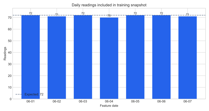
June 4 has 70 readings, while June 2 and June 7 have 71. That does not automatically make the data unusable. It tells you where to investigate and lets you choose a clear policy: accept small gaps, remove incomplete days, or add a missingness feature. The chart supports that decision; it does not make it for you.

If you prefer to inspect this query in pandas, the DataTweets guide to pandas and SQLite shows how read_sql_query turns a SQL result into a DataFrame.

Verify that late data does not change the stored snapshot

Suppose a reading for June 10 arrives after run 1 is complete. Add it to the raw table, then count the already stored feature rows:

connection.execute(
    "INSERT INTO sensor_readings VALUES (?, ?, ?, ?, ?)",
    (9999, "north", "2026-06-10 12:30:00", 24.1, 57.0),
)

after_late_insert = connection.execute(
    "SELECT COUNT(*) FROM daily_features WHERE run_id = ?",
    (run_id,),
).fetchone()[0]

print("feature rows after late insert:", after_late_insert)
connection.rollback()
connection.close()

feature rows after late insert: 21

The existing snapshot stays at 21 rows because it is a stored result, not a live view. The cutoff also means this June 10 reading would be excluded if we repeated the same feature query for run 1. A future build can use a later cutoff and a new run_id; run 1 remains available for reproducing the original experiment.

This example follows an append-only convention: completed runs are never updated or deleted. The schema does not enforce that convention by itself. In a production system, restrict write permissions or add database rules that prevent changes to completed runs.

This is also a basic defense against data leakage, which happens when training features contain information that would not have been available at prediction time. A cutoff does not prevent every form of leakage, but it gives time-based projects a clear boundary to test.

Common mistakes and troubleshooting

The script fails with OperationalError: near "STRICT". Your SQLite runtime is older than 3.37.0. Check it with print(sqlite3.sqlite_version). Upgrade Python to get a newer bundled SQLite, or remove STRICT while keeping the other constraints. Do not remove validation without replacing it.

A valid-looking timestamp falls on the wrong side of the cutoff. ISO timestamps compare correctly as text only when every value uses the same sortable format, such as YYYY-MM-DD HH:MM:SS, and the same time zone. Normalize timestamps before loading. For multi-region systems, UTC is usually the simplest shared standard.

Rerunning the script creates duplicate features. The primary key prevents two rows with the same (run_id, zone, feature_date). For a fresh local exercise, delete the database before rebuilding. In a real pipeline, create a new run or make the build explicitly replace only an incomplete run.

PRAGMA foreign_keys = ON seems to do nothing. Set it immediately after opening every connection and before starting a transaction. SQLite foreign-key enforcement is configured per connection.

A snapshot has the expected row count but poor coverage. Row counts at the feature level cannot reveal every missing raw reading. Keep reading_count, compare it with the expected frequency, and inspect a coverage chart or validation query.

The database remains locked after an error. Roll back the failed transaction and close the connection. During development, place database work in try/finally or use contextlib.closing so cleanup still happens when a statement fails.

Recap

A reproducible training table needs more than a saved CSV. It needs a boundary and a record of how it was made:

• Keep raw readings separate from derived model features.
• Reject impossible values with database constraints.
• Record a cutoff and feature definition under a run_id.
• Build features from rows before that cutoff.
• Store feature rows so later raw data cannot change the old snapshot.
• Validate source counts, feature counts, coverage, and database integrity.

The durable mental model is raw data → recorded run → fixed features. Once that chain exists, model experiments can refer to a specific snapshot instead of an unnamed, changing table.

For a larger-than-memory source, continue with streaming a large CSV into SQLite. It uses batches to keep memory bounded before the snapshot step shown here.