Route Support Tickets with Naive Bayes in Python

A support team receives short messages about payments, accounts, and software errors. Someone must read each message before sending it to the right queue. A text classifier can suggest that first destination. It does not need to write a reply or understand every detail. It only needs to choose among a few known categories.

In this tutorial, you will build that classifier with Multinomial Naive Bayes. This is a fast probability-based method that works well as a baseline for word-count data. You will turn text into numbers, keep test data separate, evaluate the results, and inspect uncertain predictions. If you are new to model training, the first machine learning model tutorial explains the wider fit, predict, and evaluate workflow.

What You Need Before You Begin

You need Python 3.11 or newer and basic knowledge of Python lists and tables. You do not need prior knowledge of probability or natural language processing (NLP). NLP means using software to work with human language.

Create a project folder, open a terminal in it, and install the three packages used here:

python -m pip install pandas scikit-learn matplotlib

The published results were tested with Python 3.13.2, pandas 3.0.3, scikit-learn 1.9.0, and Matplotlib 3.11.0. The complete synthetic dataset is available at /datasets/blog/route-support-tickets-naive-bayes/support-tickets.csv. It contains no real customer information.

The dataset is original DataTweets teaching material released under CC0 1.0. It has 90 fictional tickets: 30 each for account, billing, and technical. The examples were designed to have clear wording so that each processing step is easy to inspect. They are not evidence that the model will reach the same score on real support data.

How Word-Count Naive Bayes Works

Multinomial Naive Bayes cannot accept raw sentences directly. First, CountVectorizer builds a vocabulary, which is the set of tokens found in the training text. A token is a text unit; here it is usually one word. The vectorizer then creates one numeric column per token and counts how often each token appears in each ticket.

Suppose the training data often contains invoice in billing tickets and password in account tickets. Naive Bayes learns that these observations support different categories. For a new ticket, it combines three kinds of information:

1. The prior: how common each category was in the training data.
2. The word evidence: how often the ticket’s words occurred in each category.
3. Smoothing: a small added count that prevents an unseen word-category pair from making a category’s score zero.

The word naive refers to the model’s simplifying assumption that features contribute independently once the category is known. Real words are not independent. For example, reset and password often appear together. The assumption is still useful because it makes training quick and often gives a strong first model.

Scikit-learn’s Naive Bayes guide defines Multinomial Naive Bayes for discrete features such as word counts. Its smoothing value alpha=1.0 is Laplace smoothing. The CountVectorizer reference documents how text becomes a sparse count matrix. Sparse means the matrix stores mainly the nonzero values, which saves memory when most tickets use only a small part of the vocabulary.

Load and Inspect the Ticket Data

Begin by loading the CSV with pandas. Looking at a few rows before modeling catches wrong column names, missing labels, and unexpected text.

import pandas as pd

tickets = pd.read_csv("support-tickets.csv")
print(tickets.head(3).to_string(index=False))
print("shape:", tickets.shape)
print(tickets["category"].value_counts().sort_index())

 ticket_id                                         text category
      1001 I cannot sign in after changing phones.  account
      1002 I cannot sign in since this morning.      account
      1003 I cannot sign in on the mobile app.        account
shape: (90, 3)
category
account      30
billing      30
technical    30
Name: count, dtype: int64

Each row has an identifier, the ticket text, and the correct destination. The equal counts make this lesson easier to read because no category dominates the data. Real queues are rarely this balanced, so you should always check label counts in your own project.

Split Before Learning the Vocabulary

A training set teaches the model. A test set checks it on rows it did not use for training. Split the raw text before fitting the vectorizer. Otherwise, the vocabulary can learn information from test messages. That mistake is a form of data leakage, which means information from the evaluation data enters model training.

The next code reserves 25% of the rows for testing. stratify keeps all three categories represented in similar proportions.

from sklearn.model_selection import train_test_split

train_text, test_text, train_labels, test_labels = train_test_split(
    tickets["text"],
    tickets["category"],
    test_size=0.25,
    random_state=27,
    stratify=tickets["category"],
)

print("training tickets:", len(train_text))
print("test tickets:", len(test_text))

training tickets: 67
test tickets: 23

random_state=27 fixes the shuffle, so the same rows enter each set every time. Reproducibility is important when you compare code, metrics, or model settings.

Build One Safe Text Pipeline

A scikit-learn Pipeline passes data through steps in order. Here, the vectorizer creates counts and the classifier learns from those counts. Keeping both steps together also ensures that prediction applies the same vocabulary used during training.

We will count both single words and two-word sequences by setting ngram_range=(1, 2). A sequence of adjacent tokens is an n-gram. A one-token n-gram is a unigram, while a two-token n-gram is a bigram. Bigrams let the model distinguish phrases such as reset link from either word alone.

from sklearn.feature_extraction.text import CountVectorizer
from sklearn.naive_bayes import MultinomialNB
from sklearn.pipeline import Pipeline

model = Pipeline([
    ("counts", CountVectorizer(ngram_range=(1, 2))),
    ("classifier", MultinomialNB(alpha=1.0)),
])

model.fit(train_text, train_labels)
print(model)

Pipeline(steps=[('counts', CountVectorizer(ngram_range=(1, 2))),
                ('classifier', MultinomialNB())])

fit performs two learning operations. The vectorizer learns its vocabulary from the 67 training tickets. The classifier then estimates category and token probabilities from the resulting counts. Scikit-learn documents this ordered transformer-estimator design in its pipeline API.

You can inspect the numeric representation without printing the whole matrix:

vectorizer = model.named_steps["counts"]
train_counts = vectorizer.transform(train_text)

print("count matrix shape:", train_counts.shape)
print("vocabulary size:", len(vectorizer.get_feature_names_out()))

count matrix shape: (67, 304)
vocabulary size: 304

The matrix has 67 rows, one per training ticket, and 304 columns, one per learned unigram or bigram. Most cells are zero because one short ticket contains few of those 304 features.

Predict Categories and Read Probabilities

Use predict when you need the chosen category. Use predict_proba when you also need the model’s estimated probability for every category. These estimates can support review rules, but they are not guarantees that a prediction is correct.

new_tickets = [
    "The reset code does not arrive when I try to sign in",
    "Why did the plan charge me again this month?",
    "Reports freeze whenever I open the dashboard",
]

predicted = model.predict(new_tickets)
probabilities = model.predict_proba(new_tickets)
labels = model.named_steps["classifier"].classes_

for text, category, scores in zip(new_tickets, predicted, probabilities):
    score_text = ", ".join(
        f"{label}={score:.3f}" for label, score in zip(labels, scores)
    )
    print(f"{category:9} | {score_text} | {text}")

account   | account=0.902, billing=0.002, technical=0.096 | The reset code does not arrive when I try to sign in
billing   | account=0.147, billing=0.810, technical=0.043 | Why did the plan charge me again this month?
technical | account=0.082, billing=0.151, technical=0.767 | Reports freeze whenever I open the dashboard

The first line has its largest value under account, so that is the prediction. Its technical probability is not zero because some words, such as does and when, can occur across categories. The three probabilities on each line sum to approximately 1.

Now consider a less specific message:

text = ["I cannot use my plan"]
print("prediction:", model.predict(text)[0])
print(dict(zip(labels, model.predict_proba(text)[0].round(3))))

prediction: billing
{'account': 0.024, 'billing': 0.971, 'technical': 0.005}

The model assigns a high probability to billing because plan appears mainly in billing examples. A person may still need to ask whether the customer has a payment problem or a technical access problem. The estimate reflects patterns in the training data; it does not show whether the message contains enough real-world detail.

Evaluate the Held-Out Tickets

Never judge a classifier only from examples chosen after you see its output. Predict all 23 held-out labels, then compare them with the known answers.

from sklearn.metrics import classification_report, confusion_matrix

test_predictions = model.predict(test_text)

print(confusion_matrix(test_labels, test_predictions, labels=labels))
print(classification_report(test_labels, test_predictions, zero_division=0))

[[8 0 0]
 [0 7 0]
 [0 0 8]]
              precision    recall  f1-score   support

     account       1.00      1.00      1.00         8
     billing       1.00      1.00      1.00         7
   technical       1.00      1.00      1.00         8

    accuracy                           1.00        23

The confusion matrix places actual categories in rows and predicted categories in columns. All 23 counts lie on the main diagonal, so this particular split has no errors.

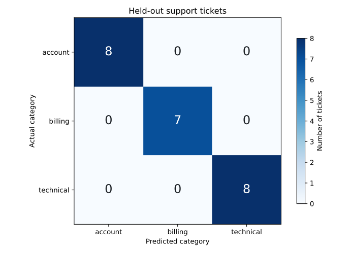
Precision asks how many tickets predicted as a category truly belonged there. Recall asks how many tickets that truly belonged to a category the model found. Both are 1.00 here because the synthetic wording is regular and the categories are distinct.

Do not read 1.00 as a production promise. Several tickets share structured phrases, and the small test set comes from the same generation rules as the training set. A real evaluation should include new writing styles, spelling errors, mixed topics, rare categories, and tickets collected after deployment. The value of this result is narrower: it verifies that the complete pipeline behaves correctly on its controlled teaching data.

Common Mistakes and Troubleshooting

You fit the vectorizer before the split. Calling fit_transform on all text lets the vocabulary see the test set. Put CountVectorizer inside a pipeline and fit the pipeline only on train_text.

You pass negative values to Multinomial Naive Bayes. This estimator expects non-negative features such as counts. Standard scaling can create negative numbers and is not appropriate for this count pipeline. Use CountVectorizer or another non-negative representation.

A new ticket contains words outside the vocabulary. The vectorizer ignores unseen tokens. If every useful token is unseen, the prediction relies mostly on learned category priors. Log these cases and retrain with representative labeled examples.

You remove too many words. Generic stop-word lists can remove short words that matter in a specific domain. Start without stop-word removal, inspect errors, and change preprocessing only when validation results support it. For preparation steps before modeling, see cleaning text data for NLP.

A high estimated probability is treated as certainty. Probability estimates can be poorly calibrated, especially on small datasets or data whose patterns have changed. Send low-probability or business-critical predictions to a person for review. Test any routing threshold on separate validation data.

One ticket contains two valid topics. This tutorial assumes exactly one category per ticket. A message about a failed payment and a locked account breaks that assumption. You can define a priority rule, allow multiple labels with a different method, or ask a person to route mixed cases.

Recap and a Practical Next Step

You built a complete text-routing baseline:

1. Load labeled ticket text and inspect the category balance.
2. Split raw text before any vocabulary learning.
3. Convert words and short phrases into non-negative counts.
4. Fit MultinomialNB inside one reusable pipeline.
5. Read predicted categories together with their probabilities.
6. Evaluate every held-out ticket with a confusion matrix, precision, and recall.

The durable mental model is simple: words become counts, counts provide evidence for each category, and the strongest combined evidence becomes the prediction. The model is a routing assistant, not an authority. A useful next experiment is to collect realistic, safely anonymized tickets, label them consistently, and compare this baseline with a model that uses TF-IDF features. Keep the same untouched test set so the comparison remains fair.