Save and Reload a Neural Network Pipeline in Python

A trained model is useful only if another Python process can reuse it. If the fitted object exists only in memory, it disappears when the process ends. The next process would have to repeat training, which takes time and may produce different weights.

Saving only the neural network is also incomplete. The network in this tutorial expects scaled numbers. A future prediction must use the same feature order, means, and standard deviations that were learned during training. A newly fitted scaler would change the input values and could change the prediction.

This tutorial solves that problem by putting a scaler and a neural network in one scikit-learn Pipeline. We will train the pipeline for a regression task, save the whole fitted object with joblib, reload it, and verify that every test prediction remains identical. Regression means predicting a number, such as a delivery time, rather than a class.

If neural-network layers and activations are new to you, start with Neural Network Classification in Python. That tutorial develops the basic network mental model. Here, the focus is the path from a trained model to a reusable model file.

Prerequisites and Setup

You need Python 3.11 or newer and basic experience with pandas DataFrames. A DataFrame is a table in which rows are observations and columns are variables. Create a virtual environment, activate it, and install the packages used below:

python -m venv .venv
source .venv/bin/activate
python -m pip install numpy pandas scikit-learn matplotlib joblib

The verified run used Python 3.13.2, NumPy 2.5.1, pandas 3.0.3, scikit-learn 1.9.0, Matplotlib 3.11.0, and joblib 1.5.3. Model files are sensitive to package versions, so recording this environment is part of the workflow.

Mental Model: The Complete Model Is More Than Its Weights

Our model receives seven route features. Their scales differ: priority_service is either 0 or 1, while warehouse_queue_min can reach 30. A neural network usually trains more reliably when its numeric inputs have comparable scales.

StandardScaler learns one mean and standard deviation for every feature. It transforms each value by subtracting that feature’s training mean and dividing by its training standard deviation. The neural network learns from these transformed values, not from the original table.

The prediction path therefore has two fitted parts:

1. The scaler stores the training statistics and transforms a new row.
2. The network stores its learned parameters and converts the scaled row into a time estimate.

Saving the full pipeline keeps these parts together. scikit-learn’s Pipeline guide also explains that the pipeline exposes the final estimator’s predict() method. Calling pipeline.predict(new_data) applies the scaler first and the neural network second.

Load an Original Synthetic Dataset

The example uses 1,600 fictional courier routes generated with NumPy and random seed 73. It is original synthetic data released under CC0 1.0. No rows describe real couriers, customers, or delivery operations. Use it to learn the workflow, not to make operational promises.

The CSV is available as courier_route_times.csv. Load it and inspect three small rows before selecting features:

import pandas as pd

route_data = pd.read_csv(
    "https://datatweets.com/datasets/blog/"
    "save-load-neural-network-pipeline-python/courier_route_times.csv"
)

print(route_data.shape)
print(route_data.head(3).to_string(index=False))

(1600, 9)
route_id  distance_km  parcel_weight_kg  planned_stops  traffic_index  rain_mm  warehouse_queue_min  priority_service  delivery_minutes
   R0001        16.27              7.31              4          0.640     0.00                 1.58                 0              61.2
   R0002        10.40              3.69              1          0.870     2.69                 1.53                 0              58.5
   R0003         9.33              3.79             10          0.571     1.47                 2.21                 0              68.9

Each row has a route identifier, seven numeric input features, and the delivery_minutes target. A feature is an input used to make a prediction. The target is the value we want the model to learn to predict. We will not use route_id because this arbitrary identifier contains no route measurement.

Reserve an Untouched Test Set

Define the feature list explicitly. This makes the expected column order visible and prevents the identifier or target from entering the model by accident. Then reserve 20% of the rows for a final test:

from sklearn.model_selection import train_test_split

feature_columns = [
    "distance_km",
    "parcel_weight_kg",
    "planned_stops",
    "traffic_index",
    "rain_mm",
    "warehouse_queue_min",
    "priority_service",
]

X = route_data[feature_columns]
y = route_data["delivery_minutes"]

X_train, X_test, y_train, y_test = train_test_split(
    X,
    y,
    test_size=0.20,
    random_state=73,
)

print(X_train.shape, X_test.shape)

(1280, 7) (320, 7)

The network can use the 1,280 training rows to adjust its weights. The 320 test rows remain outside both fitting and early stopping. This separation gives us a final evaluation on routes that did not influence the fitted pipeline.

Build One Pipeline for Scaling and Prediction

Now connect StandardScaler to MLPRegressor. An MLP, or multilayer perceptron, is a feed-forward neural network made of connected layers. The two hidden layers below contain 32 and 16 units. ReLU activations let those layers represent non-linear relationships, such as traffic having a larger effect on long routes.

from sklearn.neural_network import MLPRegressor
from sklearn.pipeline import Pipeline
from sklearn.preprocessing import StandardScaler

pipeline = Pipeline([
    ("scale", StandardScaler()),
    ("network", MLPRegressor(
        hidden_layer_sizes=(32, 16),
        activation="relu",
        solver="adam",
        alpha=0.001,
        batch_size=64,
        learning_rate_init=0.002,
        max_iter=800,
        early_stopping=True,
        validation_fraction=0.15,
        n_iter_no_change=25,
        random_state=73,
    )),
])

solver="adam" selects the algorithm that updates the weights. alpha discourages very large weights. max_iter=800 is an upper limit, not a requirement to run all 800 epochs. An epoch is one pass over the training rows.

With early_stopping=True, MLPRegressor holds back 15% of its training input as validation data. Validation data does not update the weights. The estimator stops after 25 epochs without enough validation-score improvement. The current MLPRegressor documentation describes these settings and notes that its validation score for regression is R².

Fit the whole pipeline, then read the fitted network’s training summary:

pipeline.fit(X_train, y_train)

network = pipeline.named_steps["network"]
print("epochs:", network.n_iter_)
print("best validation R2:", round(network.best_validation_score_, 4))

epochs: 358
best validation R2: 0.9682

Training stopped at epoch 358, well before the 800-epoch limit. The validation R² helped decide when to stop, so it is part of the model-fitting process rather than an independent final result.

Evaluate Before Saving

Predict the untouched test routes and compare the results with their known synthetic targets. Mean absolute error, or MAE, is the average absolute difference between a prediction and its target. R² compares the model’s squared errors with those of a constant prediction equal to the target mean. An R² of 1 is perfect, 0 is no better than that mean prediction, and a negative value is worse.

import numpy as np
from sklearn.metrics import mean_absolute_error, r2_score

test_predictions = pipeline.predict(X_test)
test_mae = mean_absolute_error(y_test, test_predictions)
test_r2 = r2_score(y_test, test_predictions)

baseline_predictions = np.repeat(y_train.median(), len(y_test))
baseline_mae = mean_absolute_error(y_test, baseline_predictions)

print(f"test MAE: {test_mae:.2f} minutes")
print(f"test R2: {test_r2:.3f}")
print(f"median baseline MAE: {baseline_mae:.2f} minutes")

test MAE: 3.87 minutes
test R2: 0.976
median baseline MAE: 26.24 minutes

The model’s predictions differ from the generated targets by 3.87 minutes on average. The median baseline misses by 26.24 minutes. On this controlled test set, the large gap shows that the network captured the synthetic pattern. It says nothing about performance on real delivery data.

The chart shows all 320 test predictions. The dashed diagonal marks perfect agreement. Points above it are overestimates, and points below it are underestimates.

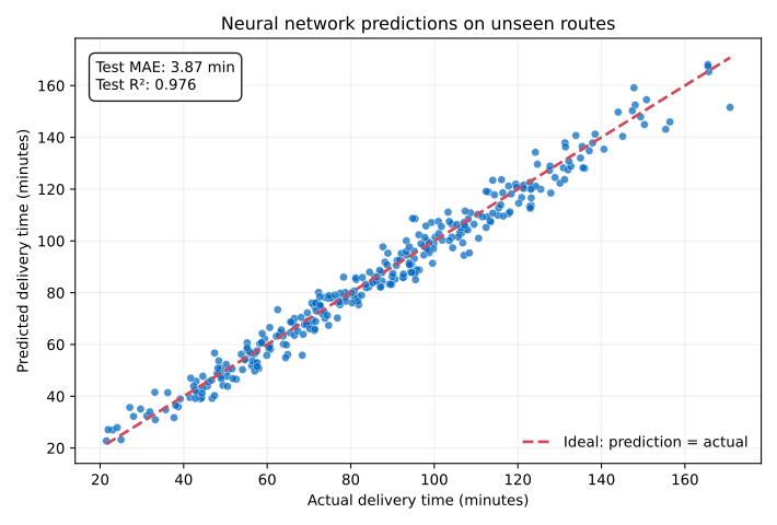
The points follow the diagonal across short and long routes. A few wider gaps remain, which is expected because the dataset generator adds random variation that the features cannot explain.

Save and Reload the Whole Pipeline

joblib.dump() writes the fitted Python object to a file. Save pipeline, not network, so the scaler’s learned means and standard deviations travel with the neural-network weights:

import joblib

model_path = "courier_duration_pipeline.joblib"
joblib.dump(pipeline, model_path)

reloaded_pipeline = joblib.load(model_path)
reloaded_predictions = reloaded_pipeline.predict(X_test)

maximum_difference = np.max(
    np.abs(test_predictions - reloaded_predictions)
)
print("maximum prediction difference:", maximum_difference)

maximum prediction difference: 0.0

The maximum difference is exactly zero. This check matters more than merely confirming that the file exists: it verifies that saving and loading preserved the fitted pipeline’s output for every test row in the tested environment.

joblib uses Python’s pickle system. Loading a joblib file can run code, so load only files that you created or obtained from a trusted source. Scikit-learn’s current model persistence guide also warns that loading a model with different scikit-learn or dependency versions is unsupported. Keep the training code, dataset record, and package versions with the model artifact.

Predict One New Route

The reloaded object accepts the same seven-column DataFrame as the original pipeline. Build one new fictional route with every required feature, then call predict():

new_route = pd.DataFrame([{
    "distance_km": 12.5,
    "parcel_weight_kg": 3.2,
    "planned_stops": 5,
    "traffic_index": 0.68,
    "rain_mm": 2.0,
    "warehouse_queue_min": 7.0,
    "priority_service": 0,
}])

predicted_minutes = reloaded_pipeline.predict(new_route)[0]
print(f"predicted delivery time: {predicted_minutes:.1f} minutes")

predicted delivery time: 67.2 minutes

For prediction, supply the feature values in their original units. Do not scale them manually because the stored StandardScaler already does that inside the pipeline. The result is a model estimate for a synthetic scenario, not a guaranteed arrival time.

Common Mistakes and Troubleshooting

Saving only the final estimator. pipeline.named_steps["network"] contains the neural network, but it cannot transform the original feature values by itself. Save the full pipeline so future inputs follow the same fitted scaling step.

Fitting again after loading. Calling fit() changes the learned pipeline instead of using it for prediction. Fitting a separate new scaler also changes the numbers sent to the fixed network. When you only want predictions, call predict() on the loaded pipeline directly.

Changing column names or order. The fitted pipeline expects the same seven named features. Build prediction DataFrames with the training names and check that no value is missing. scikit-learn raises an error when feature names do not match, which is safer than silently using the wrong input.

Evaluating after seeing test results many times. If you repeatedly change model settings because of the test score, the test set becomes an informal validation set. Choose settings with training and validation data, then use the test set for one final report.

Loading an untrusted joblib file. Treat a model file like executable code. Do not load attachments or downloaded files merely because their extension is .joblib.

Ignoring version records. A file that loads today may not load after a major package upgrade. Record the full environment, including Python, NumPy, SciPy, scikit-learn, and joblib versions. Keep reproducible training code so you can rebuild the artifact in a new environment.

Recap

The durable idea is simple: prediction depends on the complete fitted path, not only on neural-network weights.

• Split the data before fitting so the test rows remain untouched.
• Put StandardScaler and MLPRegressor in one pipeline.
• Evaluate the fitted pipeline against both an unseen test set and a simple baseline.
• Save the whole pipeline with joblib.dump().
• Reload only trusted files in a matching package environment.
• Compare predictions before and after loading to verify that persistence worked.

For a small local Python project, this creates a clear handoff from training to later prediction. A production system needs additional controls, including artifact signing, access restrictions, input validation, monitoring, and a planned process for retraining.