Build and Backtest a Seasonal Naive Forecast in Python

A warehouse needs to decide how many packing stations to prepare each morning. Recent order volume helps, but yesterday may be a poor guide. A busy Monday can follow a quiet Sunday even when nothing unusual has happened.

This tutorial builds a seasonal naive forecast: a prediction that reuses the value from the same position in the previous cycle. For daily warehouse data with a weekly cycle, next Monday’s forecast is the previous Monday’s order count.

We will create three simple forecasts with pandas, backtest them on 28 later days, and compare their errors. The main goal is not to find the most advanced model. It is to build a trustworthy baseline that a more complex forecasting model should beat.

If you first want to explore rather than predict a repeating pattern, see how to find weekly seasonality with pandas. That tutorial separates completed history into a trend, weekday effect, and residual. Here, every prediction uses only information that was available before the predicted day.

Prerequisites and setup

You should be able to run a Python script or notebook cell. You do not need forecasting experience. A time series is a sequence of observations arranged by time, such as one order count per day.

Create a virtual environment to keep this lesson’s packages separate from your other projects. Then install the required packages:

python -m venv .venv
source .venv/bin/activate
python -m pip install numpy pandas matplotlib

On Windows PowerShell, activate the environment with .venv\Scripts\Activate.ps1. The published artifacts were executed with Python 3.13.2, NumPy 2.5.1, pandas 3.0.3, and Matplotlib 3.11.0.

Download warehouse_orders.csv into your working folder. It has 224 consecutive daily order counts from 6 January through 17 August 2025. The warehouse and every count are fictional. The dataset was generated with a fixed random seed and is released under CC0-1.0, so you may reuse it without restriction.

The historical dates only make the exercise concrete. They do not describe a real organization.

The mental model: repeat the relevant past

A baseline forecast is a simple reference method. It tells us how much accuracy is available from an obvious rule before we add model complexity.

We will compare three rules:

1. Yesterday: use the previous day’s count.
2. Trailing mean: use the mean of the previous seven days.
3. Seasonal naive: use the count from seven days ago.

The seasonal rule can be written as:

forecast for day t = observed value at day t - 7

The number 7 is the seasonal period, meaning the number of observations in one repeating cycle. It is seven only because this dataset has one observation per day and a weekly operating pattern. For monthly data with a yearly pattern, the period would usually be 12 observations.

“Naive” does not mean useless. It means the rule does not fit model parameters from training data. When a weekly pattern is strong and changes slowly, the same weekday last week can be a difficult baseline to beat.

Our warehouse makes one forecast each morning, after the previous day’s actual count is known. This is a one-day-ahead forecast: each prediction is for the next day only. That detail controls which past observations the code may use.

Load the data and verify the calendar

First, parse date as a datetime value, make it the row index, and print a small sample. A DatetimeIndex is a date-aware set of row labels.

import pandas as pd

orders = pd.read_csv("warehouse_orders.csv", parse_dates=["date"])
orders = orders.set_index("date").sort_index()

print(orders.head(8).to_string())
print("\nrows:", len(orders))
print("frequency:", pd.infer_freq(orders.index))
print("duplicate dates:", orders.index.duplicated().sum())
print("missing counts:", orders["orders_to_pack"].isna().sum())

            orders_to_pack
date                      
2025-01-06             208
2025-01-07             197
2025-01-08             206
2025-01-09             196
2025-01-10             202
2025-01-11             151
2025-01-12             142
2025-01-13             211

rows: 224
frequency: D
duplicate dates: 0
missing counts: 0

D means that pandas found a daily frequency. There are no duplicate dates or missing counts. This check is essential: shift(7) means seven rows earlier, so it represents one week only when the rows form a complete, correctly ordered daily sequence.

The first eight rows already show why yesterday can fail. Sunday has 142 orders, followed by 211 on Monday. The previous Monday, 208, is a more relevant comparison.

If a real dataset has missing dates, first use pandas asfreq("D") to conform it to a daily index. The inserted rows will contain missing values. Investigate them rather than automatically replacing them with zero; a missing record and a real zero-order day mean different things.

Create forecasts with shift and rolling

Now place the actual series and all three predictions in one DataFrame. Each expression must exclude the value being predicted.

series = orders["orders_to_pack"]
forecasts = pd.DataFrame({"actual": series})

forecasts["yesterday"] = series.shift(1)
forecasts["trailing_7_day_mean"] = series.shift(1).rolling(7).mean()
forecasts["same_weekday_last_week"] = series.shift(7)

print(forecasts.head(10).round(1).to_string())

            actual  yesterday  trailing_7_day_mean  same_weekday_last_week
date                                                                      
2025-01-06     208        NaN                  NaN                     NaN
2025-01-07     197      208.0                  NaN                     NaN
2025-01-08     206      197.0                  NaN                     NaN
2025-01-09     196      206.0                  NaN                     NaN
2025-01-10     202      196.0                  NaN                     NaN
2025-01-11     151      202.0                  NaN                     NaN
2025-01-12     142      151.0                  NaN                     NaN
2025-01-13     211      142.0                186.0                   208.0
2025-01-14     202      211.0                186.4                   197.0
2025-01-15     194      202.0                187.1                   206.0

shift moves earlier values onto later rows when you do not pass a freq argument. Here, shift(1) puts yesterday’s observation on today’s row. For the trailing mean, shifting must happen before calculating the rolling average. The 13 January forecast averages 6–12 January and does not include 13 January’s actual value.

shift(7) aligns the previous week’s same weekday with the current row. On 13 January it predicts 208, the actual value from Monday 6 January.

The missing values at the beginning are expected. On the first day, there is no yesterday. The seasonal forecast needs one complete week of earlier observations. pandas uses NaN for those unavailable numeric values.

Backtest on later dates

A backtest simulates how a forecast would have worked using historical data. We will reserve the final 28 days as a test period. All three methods predict the same dates, which makes the comparison fair.

The next code selects the test rows and confirms that every method has a prediction for every test date. It does not tune or adjust any method after seeing the test errors.

test_start = series.index[-28]
test = forecasts.loc[test_start:].copy()

print("test starts:", test_start.date())
print("test days:", len(test))
print("missing test predictions:", test.drop(columns="actual").isna().sum().sum())
print(test.head(8).round(1).to_string())

test starts: 2025-07-21
test days: 28
missing test predictions: 0
            actual  yesterday  trailing_7_day_mean  same_weekday_last_week
date                                                                      
2025-07-21     230      170.0                215.3                   247.0
2025-07-22     239      230.0                212.9                   230.0
2025-07-23     223      239.0                214.1                   237.0
2025-07-24     224      223.0                212.1                   222.0
2025-07-25     209      224.0                212.4                   214.0
2025-07-26     178      209.0                211.7                   187.0
2025-07-27     168      178.0                210.4                   170.0
2025-07-28     234      168.0                210.1                   230.0

Read the first row carefully. For Monday 21 July, the yesterday method predicts only 170 because Sunday was quiet. The seasonal method uses the previous Monday and predicts 247. Its error is 17 orders, while the yesterday method’s error is 60.

The 28 July seasonal forecast uses the actual count from 21 July. That is valid for this one-day-ahead workflow because the 21 July value was already known before the forecast for 28 July was made. It would not be valid in a forecast created four weeks in advance.

Compare errors with mean absolute error

We need one measure that summarizes 28 daily misses. Mean absolute error (MAE) is the average distance between actual and predicted values, ignoring whether a forecast was too high or too low. Lower is better.

absolute error = |actual - forecast|
MAE = mean of all absolute errors

The following function calculates MAE in units of orders, then applies it to each prediction column:

def mae(actual, predicted):
    return (actual - predicted).abs().mean()

scores = pd.Series({
    "Yesterday": mae(test["actual"], test["yesterday"]),
    "Trailing 7-day mean": mae(
        test["actual"], test["trailing_7_day_mean"]
    ),
    "Same weekday last week": mae(
        test["actual"], test["same_weekday_last_week"]
    ),
}).sort_values()

print(scores.round(2).to_string())

Same weekday last week     8.79
Trailing 7-day mean       20.79
Yesterday                 21.82

The seasonal naive forecast misses by 8.79 orders per day on average. The trailing mean misses by 20.79, and yesterday misses by 21.82. On this synthetic series, preserving the weekday position matters much more than using the most recent value.

This result does not prove that seasonal naive forecasting will win on another dataset. It establishes the score that a more complex model must beat under the same backtest procedure.

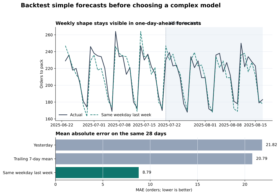
In the top panel, the dashed forecast follows the repeated Monday-to-weekend shape. It does not match every daily movement, but it keeps high weekdays and low weekends in the right part of the week. The lower panel makes the comparison direct: all bars use the same dates and the same error unit.

What this backtest does not tell you

The test answers a narrow operational question: if each morning we know all counts through yesterday, how well does each rule predict today?

It does not evaluate a 28-day forecast made at one fixed date. After the first week of the test period, shift(7) uses actual values from within that test period. That is correct for rolling one-day-ahead forecasts, but those actuals would be unavailable when planning four weeks at once.

For a fixed four-week forecast, one simple seasonal rule would repeat the final seven observed training values four times. That is a different task and should receive its own backtest.

The backtest also covers only four weeks. Real evaluations should include enough cycles to represent changing demand, unusual events, and different parts of the year. A single metric can hide whether errors cluster on Mondays, weekends, or high-volume days, so inspect a plot and row-level errors as well.

Common mistakes and troubleshooting

Using rolling(7).mean() before shift(1). That includes today’s actual count in today’s forecast. The error will look better because future information leaked into the prediction. Shift first, then calculate the rolling mean.

Treating seven rows as seven days without checking dates. Missing or duplicate dates break that assumption. Sort the index, check duplicates, and verify the frequency before using row shifts.

Choosing 7 only because the data is daily. Daily data can have other patterns. A call center may repeat weekly, electricity demand may have both daily and weekly cycles, and a process may have no stable seasonality. Use domain knowledge and plots to choose a period.

Calling a rolling backtest a long-range forecast. In this lesson, each new actual becomes available before the next prediction. State the forecast horizon and update schedule so readers know what information each prediction uses.

Comparing methods on different dates. Missing predictions can silently change the rows used by a metric. Build one test table, check it for missing values, and score every method on the same dates.

Assuming the lowest MAE is automatically deployable. A useful operational forecast also needs fresh data on time, monitoring, and a response when inputs are missing. Accuracy is one requirement, not the whole system.

Expecting a baseline to explain causes. The seasonal rule predicts from repetition. It does not know about promotions, staffing, closures, or weather. A large error is a reason to investigate, not proof of one cause.

Recap and next step

A seasonal naive forecast reuses the value from the same position in the previous cycle. For complete daily data with a weekly pattern, series.shift(7) creates a clear one-day-ahead baseline.

The durable workflow is:

1. Verify that dates are ordered, unique, and regularly spaced.
2. Define the forecast horizon and what information is available at prediction time.
3. Create simple rules without including the target day’s actual value.
4. Reserve later dates for a backtest.
5. Compare every method on those same dates with an interpretable metric.

In this fictional warehouse dataset, the weekly baseline reached 8.79 orders MAE and clearly beat the yesterday and trailing-mean rules. The important result is not that exact score. It is the honest reference point. Before adopting a complex forecasting model, require it to beat the seasonal baseline on the same future-like test.

As a next step, calculate errors by weekday. If one weekday is consistently underpredicted, the weekly pattern may be changing. You can then test a trend-adjusted seasonal method or a statistical seasonal model while keeping this baseline and backtest unchanged for comparison.