A laboratory builds a screening model from a training sample containing 400 routine water samples and 400 samples that required review. That balanced sample provides enough examples of both classes. However, only 5% of samples require review during normal operation. If the model treats both classes as equally common, it can send too many routine samples to a specialist.

Set the expected deployment rates with GaussianNB(priors=[0.95, 0.05]), where each value corresponds to the class in the same position of the fitted model’s classes_ array. Then use an untouched test set with the representative 5% rate to check probabilities, precision, recall, false review flags, and missed cases.

This tutorial shows why that one argument matters. You will compare a model that learns its prior from a balanced training sample with one that receives the deployment prior explicitly. The example uses fictional measurements, so it teaches the workflow rather than a real water-safety rule.

Setup and prerequisites

You need Python 3.11 or later and basic experience with Python variables and pandas tables. You should also know that a classifier maps input values to a class. If fitting and testing a classifier are new ideas, start with your first machine learning model.

Create a virtual environment and install the packages used in the executed lesson:

python -m venv .venv
source .venv/bin/activate
python -m pip install numpy pandas scikit-learn matplotlib

On Windows PowerShell, activate the environment with .venv\Scripts\Activate.ps1. The published results were executed with Python 3.13.2, NumPy 2.5.1, pandas 3.0.3, scikit-learn 1.9.0, and Matplotlib 3.11.0.

Download water-screening.csv and save it beside your Python file or notebook. This original synthetic DATATWEETS dataset is released under CC0-1.0. Its 4,800 rows were generated with the NumPy random seed 73442.

All sample IDs, measurements, and outcomes are fictional. The columns resemble laboratory screening data, but their values are not safety limits and must not guide a real environmental decision.

Load the file and inspect only a few rows first. A small preview helps you confirm the column names and units before fitting a model.

import numpy as np
import pandas as pd

screening = pd.read_csv("water-screening.csv")
print(screening.head(3).to_string(index=False))
print("shape:", screening.shape)

sample_id  turbidity_ntu  conductivity_change_pct  uv_absorbance  requires_review    split
TR-R-0399          3.715                   -0.929          0.064                1 training
TR-R-0183          3.523                   11.029          0.092                1 training
TR-N-0320          1.865                    3.355          0.038                0 training
shape: (4800, 6)

Each row contains three numeric features. A feature is an input used for prediction. The target requires_review is 1 for a sample that needs specialist review and 0 for a routine sample.

Understanding the prior before the evidence

A class prior is the probability of a class before the model examines the current features. In normal operation, the review prior is 5% because 5 out of every 100 samples require review on average. The routine prior is therefore 95%.

Gaussian Naive Bayes also learns a feature distribution for each class. In this model, Gaussian means that each numeric feature has a bell-shaped distribution within each class. The density of a new measurement under one of these distributions supplies a likelihood: evidence showing how compatible that measurement is with the class.

For each class, the model combines the starting rate and all feature evidence:

class score = class prior × feature likelihood 1 × feature likelihood 2 × ...

The model normalizes the class scores into posterior probabilities. A posterior is the updated probability after seeing the features, under the model’s assumptions. The class with the largest posterior becomes the default prediction.

The word naive describes the assumption that the features are independent after the class is known. For example, the model acts as if turbidity and ultraviolet absorbance contribute separate evidence within each class. That assumption may be inaccurate in real measurements, so you must evaluate the model on representative data.

When priors=None, scikit-learn estimates priors from the training labels. Its current GaussianNB API states that supplied priors are not adjusted to match the training data. This is useful when a sampling plan changes class proportions but still gives representative examples within each class.

Confirm the sampling mismatch

The CSV contains two predefined parts. The training archive has equal class counts. The deployment part preserves a 5% review rate and remains untouched until evaluation.

Split the rows by their recorded purpose, then count each target value:

training = screening.query("split == 'training'").copy()
deployment = screening.query("split == 'deployment'").copy()

print("training counts:")
print(training["requires_review"].value_counts().sort_index())
print("deployment counts:")
print(deployment["requires_review"].value_counts().sort_index())

training counts:
requires_review
0    400
1    400
Name: count, dtype: int64
deployment counts:
requires_review
0    3800
1     200
Name: count, dtype: int64

The balanced training sample provides enough rows to estimate how each feature behaves in both classes. Its artificial 50% review frequency should not become the model’s operational starting rate.

This design is sometimes called case-control sampling. It selects a planned number of examples from each class instead of taking a simple sample of the operating population. The design can help collect enough rare cases, but it breaks the connection between training frequency and deployment frequency.

Prepare the feature matrices and target vectors next. Keeping their names explicit makes later evaluation easier to follow.

features = [
    "turbidity_ntu",
    "conductivity_change_pct",
    "uv_absorbance",
]

X_train = training[features]
y_train = training["requires_review"]
X_test = deployment[features]
y_test = deployment["requires_review"]

Fit the balanced-prior baseline

Start with the default model. This baseline shows what happens when GaussianNB learns its prior directly from the balanced training labels.

from sklearn.naive_bayes import GaussianNB

balanced_model = GaussianNB()
balanced_model.fit(X_train, y_train)

print("class order:", balanced_model.classes_)
print("learned priors:", balanced_model.class_prior_)

class order: [0 1]
learned priors: [0.5 0.5]

The class order is important. Position 0 in class_prior_ belongs to class 0, and position 1 belongs to class 1. The model has learned equal priors because it saw 400 rows from each class.

This does not mean the fitting code failed. The model correctly described its training sample. The problem is that the sample’s class balance does not describe normal operation.

Replace the sample prior with the operational rate

Fit a second model with the same features and rows. Only the class priors change. The values must add to 1 and must follow the model’s class order: 95% for routine class 0, then 5% for review class 1.

deployment_model = GaussianNB(priors=[0.95, 0.05])
deployment_model.fit(X_train, y_train)

print("class order:", deployment_model.classes_)
print("explicit priors:", deployment_model.class_prior_)

class order: [0 1]
explicit priors: [0.95 0.05]

Changing a prior does not change the training measurements or the class-specific means and variances learned from them. It changes how much starting weight each class receives when the model combines those distributions for a prediction.

Inspect three invented samples to see the effect before calculating full test metrics. The first resembles a routine sample, the second has mixed evidence, and the third has strong review evidence.

examples = pd.DataFrame([
    {"sample": "routine-like", "turbidity_ntu": 1.9,
     "conductivity_change_pct": 1.0, "uv_absorbance": 0.042},
    {"sample": "borderline", "turbidity_ntu": 2.8,
     "conductivity_change_pct": 3.5, "uv_absorbance": 0.058},
    {"sample": "strong review signal", "turbidity_ntu": 4.1,
     "conductivity_change_pct": 9.0, "uv_absorbance": 0.088},
])

examples["balanced_probability"] = balanced_model.predict_proba(
    examples[features]
)[:, 1]
examples["deployment_probability"] = deployment_model.predict_proba(
    examples[features]
)[:, 1]

print(examples[["sample", "balanced_probability",
                "deployment_probability"]].round(3).to_string(index=False))

              sample  balanced_probability  deployment_probability
        routine-like                 0.014                   0.001
          borderline                 0.895                   0.310
strong review signal                 1.000                   1.000

The borderline sample shows the central effect. Its feature evidence is unchanged, but the review probability falls from 0.895 to 0.310 after the model starts from a realistic 5% review rate. The strong signal still overcomes the smaller prior.

Measure the effect on deployment data

A useful prior must be checked on data that reflects operation. We will compare precision, the share of review predictions that are truly review cases, with recall, the share of true review cases the model finds. We will also count false review flags and missed review cases.

The Brier score loss is the mean squared error of the predicted probabilities. Lower is better. Use it with the class-specific error counts rather than as a complete verdict.

The next helper evaluates both models on the same 4,000 untouched rows:

from sklearn.metrics import (
    brier_score_loss,
    confusion_matrix,
    precision_score,
    recall_score,
)

def evaluate(name, model):
    probability = model.predict_proba(X_test)[:, 1]
    prediction = (probability >= 0.5).astype(int)
    matrix = confusion_matrix(y_test, prediction, labels=[0, 1])
    return {
        "model": name,
        "precision": precision_score(y_test, prediction),
        "recall": recall_score(y_test, prediction),
        "false_flags": matrix[0, 1],
        "missed_reviews": matrix[1, 0],
        "brier": brier_score_loss(y_test, probability),
    }

comparison = pd.DataFrame([
    evaluate("balanced prior", balanced_model),
    evaluate("deployment prior", deployment_model),
])
print(comparison.round(4).to_string(index=False))

           model  precision  recall  false_flags  missed_reviews  brier
  balanced prior     0.5444    0.95          159              10 0.0311
deployment prior     0.9282    0.84           13              32 0.0094

With the balanced prior, 159 routine samples are sent for review. The 5% prior reduces that count to 13 and raises precision from about 54% to 93%. Its Brier score loss is also much lower on this designed deployment sample.

There is a cost: missed review cases increase from 10 to 32, so recall falls from 95% to 84%. The explicit prior is a better description of how common the class is, but it does not remove the need to choose an action rule based on the cost of each error.

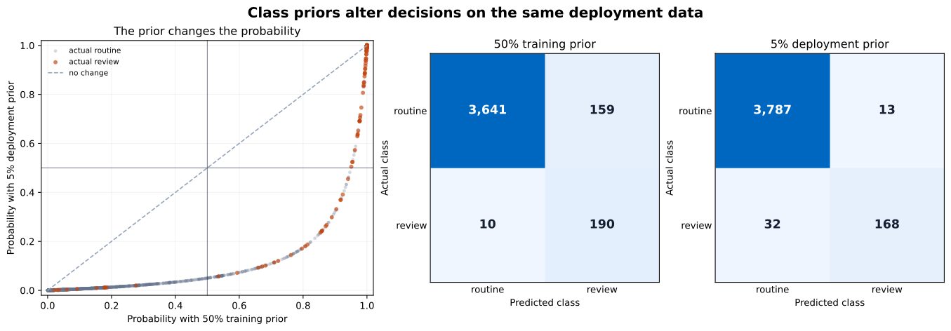
Read the left panel from the horizontal axis to the vertical axis. Points below the diagonal receive a lower review probability under the 5% prior. The confusion matrices use actual classes as rows and predicted classes as columns. Off-diagonal cells contain mistakes.

The comparison does not prove that 5% is correct for another laboratory, time period, or decision. It shows that the specified prior matches this synthetic test population and changes the trade-off in a measurable way.

Choose a prior you can defend

Do not select a prior only because it improves one test score. Estimate it from a representative operating period, a well-designed sample, or trusted domain records. Define the class and time window clearly. “Samples requiring specialist review during the next processing step” is more precise than “unusual samples.”

Check whether the rate changes by season, site, instrument, or policy. If one site has a 5% rate and another has a 20% rate, one fixed prior may not fit both. You may need separate validated models or a documented process that updates the prior.

Class priors and decision thresholds are related but answer different questions. The prior states how common a class is before the current features arrive. A threshold states when a predicted probability triggers an action. After setting a defensible prior, you can use cost-based classification thresholds in Python to choose an operating point.

Also, a correct prior does not guarantee calibrated probabilities. Calibration asks whether an event occurs in about 20% of cases that receive a predicted probability near 20%. Naive Bayes can produce extreme estimates when its independence or Gaussian assumptions are wrong. Check calibration separately; the probability calibration tutorial explains the evaluation pattern.

Common mistakes and troubleshooting

The prior values are reversed. Always fit once and inspect model.classes_. For classes [0, 1], priors=[0.95, 0.05] assigns 95% to 0. String labels are also sorted, so never rely on the order in which labels first appear in a file.

The prior array has the wrong length or total. Supply one non-negative value per class. The values must sum to 1, allowing only tiny floating-point rounding differences.

The training frequency is already representative. If rows form a suitable random sample of deployment, the default empirical prior may be appropriate. Replacing it with an unsupported number can make probabilities worse.

The balanced sample changed more than class counts. Prior correction assumes the feature examples still represent each class. If rare cases came from one instrument or one month while routine cases came from another, the learned likelihoods may also be biased. A prior cannot repair that sampling problem.

The test set was balanced too. A 50/50 test set is useful for some diagnostic questions, but it cannot show how many false flags occur in a 5% operating population. Keep at least one evaluation set with realistic class proportions.

Higher precision is called a free improvement. In this run, fewer false flags arrive with more missed review cases. Report both precision and recall, show the confusion matrix, and discuss which mistake matters more.

The same prior is used forever. Class rates can change. Monitor the current labeled rate and define when the model must be reviewed. Do not silently update a production prior without repeating evaluation.

The probabilities are treated as safety decisions. This dataset has no physical validity. A real screening system needs domain review, representative measurements, uncertainty analysis, and controls outside the classifier.

If your results differ, confirm that you used the published CSV, the listed feature order, and scikit-learn 1.9.0. Small numerical differences may occur across versions, but the supplied file and code should reproduce the reported counts under the tested environment.

Recap and next step

A class prior is the model’s starting class probability. GaussianNB learns that value from label frequencies unless you supply priors. When a balanced training archive does not match the operating population, an explicit, evidence-based prior can make the starting probabilities more realistic.

In this lesson, the balanced training sample implied a 50% review rate, while the deployment sample contained 5% review cases. Setting priors=[0.95, 0.05] reduced false review flags from 159 to 13 and Brier score loss from 0.0311 to 0.0094. Recall also fell from 95% to 84%, which is why the result must be read as a trade-off rather than a guaranteed improvement.

Keep the durable workflow: identify the sampling design, estimate a defensible operating rate, verify class order, set the prior, and evaluate on realistic untouched data. Then choose an action threshold and check calibration as separate steps.