How to Shape Time Series Data for LSTM Forecasting in PyTorch

A cold room records one sensor row every 30 minutes. The table is easy for a person to read, but an LSTM needs the rows in a different structure before it can learn from recent temperature and door activity.

To shape time series data for LSTM forecasting in PyTorch, turn each fixed-length history window into a three-dimensional tensor, or multidimensional array, with shape (samples, timesteps, features). Align each window with the next value as its target, split the windows by target time, fit scaling only on earlier rows, and pass the resulting batches to nn.LSTM(..., batch_first=True).

This tutorial builds that workflow for one-step forecasting. You will create 12-timestep windows from three sensor features, train on the first 24 days, and test on the final 6 days. You will also compare the LSTM with a last-value baseline to check whether its added complexity improves the forecasts.

Prerequisites and setup

You should be able to run a Python script or notebook cell. Basic pandas knowledge is helpful, but you do not need prior experience with LSTMs or PyTorch. An LSTM, short for long short-term memory network, is a neural network layer designed to process an ordered sequence while carrying information from earlier steps.

Create and activate a virtual environment, then install the packages used here:

python -m venv .venv
source .venv/bin/activate
python -m pip install numpy pandas matplotlib torch

On Windows PowerShell, activate the environment with .venv\Scripts\Activate.ps1. If you need a hardware-specific PyTorch command, use the selector in the official PyTorch installation guide.

The published artifacts were executed on CPU with Python 3.13.2, NumPy 2.5.1, pandas 3.0.3, Matplotlib 3.11.0, and PyTorch 2.12.0.

Download cold_room_readings.csv into your working folder. It contains 1,440 half-hour readings, or 30 complete days. The cold room, temperatures, and door events are synthetic and were created with a fixed seed for this lesson. The dataset is released under CC0-1.0, so you may reuse it without restriction.

If you are new to neural-network training, the practical introduction to TensorFlow and Keras explains layers, loss, optimizers, and epochs. This lesson uses PyTorch, but those ideas are shared by both frameworks.

Mental model: one window becomes one sample

A normal time-series table has one row per timestamp. An LSTM training input adds another dimension: several consecutive rows become one sample, meaning one example from which the model learns.

Our first sample uses the readings from midnight through 05:30 to predict room temperature at 06:00:

12 input rows × 3 features  ->  1 next-temperature target
00:00 through 05:30        ->  room temperature at 06:00

The three tensor dimensions have separate meanings:

1. Samples are the sliding windows available for training or testing.
2. Timesteps are the ordered rows inside one window. Here, 12 half-hour steps represent 6 hours.
3. Features are the values at each step: room temperature, outside temperature, and door-open minutes.

One sample therefore has shape (12, 3). When training groups 64 samples into one batch, the shape becomes (64, 12, 3). PyTorch’s nn.LSTM documentation calls this (batch, sequence, feature) order when batch_first=True.

The target is not inside the window. It is the room temperature on the next row. Keeping that boundary clear prevents the model from seeing the answer among its inputs.

The LSTM processes the 12 rows from oldest to newest. Its internal state can carry useful information forward, such as a recent door opening followed by a temperature rise. We will use the output from the final timestep to make one numeric prediction.

Load the readings and check the time grid

First, parse the timestamps, sort the rows, and inspect the structure. These checks matter because “12 rows” means “6 hours” only when the half-hour grid is complete.

import pandas as pd

readings = pd.read_csv("cold_room_readings.csv", parse_dates=["timestamp"])
readings = readings.sort_values("timestamp").reset_index(drop=True)

print(readings.head(5).to_string(index=False))
print("\nshape:", readings.shape)
print("frequency:", pd.infer_freq(readings["timestamp"]))
print("duplicate timestamps:", readings["timestamp"].duplicated().sum())
print("missing values:", readings.isna().sum().sum())

          timestamp  room_temp_c  outside_temp_c  door_open_minutes
2025-05-01 00:00:00        3.800          28.218                  0
2025-05-01 00:30:00        3.893          28.746                  0
2025-05-01 01:00:00        3.944          26.658                  0
2025-05-01 01:30:00        3.897          26.763                  0
2025-05-01 02:00:00        3.980          25.867                  0

shape: (1440, 4)
frequency: 30min
duplicate timestamps: 0
missing values: 0

30min confirms a regular half-hour series. There are no duplicate timestamps or missing cells. With real sensor data, do not continue until you understand gaps and duplicates. A missing reading is not the same as a zero-minute door opening.

The target is room_temp_c. We also include it as an input feature because the recent room temperature is known when the next forecast is made. Outside temperature and door activity provide extra context.

Split by time and scale without leakage

The final six days begin at row 1,152. They form the test period. We do not choose random test rows because deployment moves from earlier data toward later data.

Neural networks usually train more steadily when numeric inputs have similar scales. We will standardize each feature by subtracting its training mean and dividing by its training standard deviation. The target receives its own mean and standard deviation so we can convert predictions back to degrees Celsius.

The important detail is where those statistics come from. Calculate them from rows before the test period only:

import numpy as np

feature_names = [
    "room_temp_c",
    "outside_temp_c",
    "door_open_minutes",
]
test_start_row = 1_152

feature_values = readings[feature_names].to_numpy(dtype=np.float32)
target_values = readings["room_temp_c"].to_numpy(dtype=np.float32)

feature_mean = feature_values[:test_start_row].mean(axis=0)
feature_std = feature_values[:test_start_row].std(axis=0)
target_mean = target_values[:test_start_row].mean()
target_std = target_values[:test_start_row].std()

scaled_features = (feature_values - feature_mean) / feature_std
scaled_target = (target_values - target_mean) / target_std

Using all 30 days for scaling would let the test period influence the training transformation. That is data leakage, which means information from the evaluation period affects model development. It can make an evaluation look more reliable than it is.

Door-open minutes contain many zeros, but their training standard deviation is not zero because the training period includes door events. In a real pipeline, check for constant features before dividing. A zero standard deviation needs separate handling, such as removing that feature.

Build aligned sliding windows

Now create the three-dimensional input tensor. For each possible target row, the function takes the preceding 12 feature rows and pairs them with the target at that row.

def make_windows(features, target, lookback):
    inputs, targets, target_rows = [], [], []

    for target_row in range(lookback, len(features)):
        inputs.append(features[target_row - lookback:target_row])
        targets.append(target[target_row])
        target_rows.append(target_row)

    return (
        np.asarray(inputs, dtype=np.float32),
        np.asarray(targets, dtype=np.float32),
        np.asarray(target_rows),
    )


lookback = 12
all_x, all_y, target_rows = make_windows(
    scaled_features,
    scaled_target,
    lookback,
)

The slice ends before target_row, because Python excludes the stop position. That small rule keeps the target outside the input.

Split windows according to their target row, not according to the first row inside each window. This lets the first test target use the final 12 known training-period readings as its history:

train_mask = target_rows < test_start_row
test_mask = target_rows >= test_start_row

x_train, y_train = all_x[train_mask], all_y[train_mask]
x_test, y_test = all_x[test_mask], all_y[test_mask]

print("train X:", x_train.shape, "train y:", y_train.shape)
print("test X:", x_test.shape, "test y:", y_test.shape)

train X: (1140, 12, 3) train y: (1140,)
test X: (288, 12, 3) test y: (288,)

Read x_train.shape from left to right: 1,140 samples, 12 timesteps per sample, and 3 features per timestep. The first 12 original rows cannot be targets because they are needed as history. That is why 1,152 training rows produce 1,140 training windows.

Inspect the boundary of the first window in the original units:

print(readings.loc[:11, ["timestamp", *feature_names]].tail(3).to_string(index=False))
print("\ntarget:")
print(readings.loc[12, ["timestamp", "room_temp_c"]].to_string())

          timestamp  room_temp_c  outside_temp_c  door_open_minutes
2025-05-01 04:30:00        3.740          22.905                  0
2025-05-01 05:00:00        3.749          22.456                  0
2025-05-01 05:30:00        3.750          20.480                  0

target:
timestamp      2025-05-01 06:00:00
room_temp_c                  3.724

The visible rows are the final three timesteps of the first input. The next timestamp, 06:00, supplies the target. This manual check is one of the fastest ways to catch an off-by-one error.

Define an LSTM that returns one forecast

The model needs three input features, not 12. input_size=3 describes the width of each timestep. The lookback length is already present in the input tensor’s middle dimension.

import torch
from torch import nn

torch.manual_seed(4593884)
torch.use_deterministic_algorithms(True)
torch.set_num_threads(1)


class TemperatureLSTM(nn.Module):
    def __init__(self, feature_count):
        super().__init__()
        self.lstm = nn.LSTM(
            input_size=feature_count,
            hidden_size=16,
            batch_first=True,
        )
        self.output = nn.Linear(16, 1)

    def forward(self, inputs):
        sequence_output, _ = self.lstm(inputs)
        final_step = sequence_output[:, -1, :]
        return self.output(final_step).squeeze(-1)


model = TemperatureLSTM(feature_count=len(feature_names))

hidden_size=16 asks the LSTM to produce 16 learned values at every timestep. The expression sequence_output[:, -1, :] selects all samples, the last timestep, and all 16 hidden values. The linear layer converts those 16 values into one forecast.

The seed, deterministic-algorithm setting, and single-thread setting match the tested CPU run used for this tutorial. PyTorch’s reproducibility notes explain that identical results are not guaranteed across releases, platforms, or CPU and GPU execution. Your final decimals may differ even when the workflow is correct.

Batch the windows and train the model

TensorDataset pairs inputs and targets by their first dimension. DataLoader then returns small batches. The official PyTorch data documentation describes this automatic batching behavior.

from torch.utils.data import DataLoader, TensorDataset

train_data = TensorDataset(
    torch.from_numpy(x_train),
    torch.from_numpy(y_train),
)
generator = torch.Generator().manual_seed(4593884)
train_loader = DataLoader(
    train_data,
    batch_size=64,
    shuffle=True,
    generator=generator,
)

Shuffling training windows is acceptable here because every window contains its own ordered 12-step history. We have already made the time-based train/test split. We are not shuffling the timesteps inside a window.

Use mean squared error as the training loss and Adam as the optimizer. One epoch is one pass through all 1,140 training windows.

loss_function = nn.MSELoss()
optimizer = torch.optim.Adam(model.parameters(), lr=0.01)

for epoch in range(1, 81):
    model.train()
    loss_sum = 0.0

    for batch_x, batch_y in train_loader:
        optimizer.zero_grad()
        predictions = model(batch_x)
        loss = loss_function(predictions, batch_y)
        loss.backward()
        optimizer.step()
        loss_sum += loss.item() * len(batch_x)

    if epoch in {1, 20, 40, 60, 80}:
        mean_loss = loss_sum / len(train_data)
        print(f"epoch {epoch:>2}: scaled training MSE = {mean_loss:.6f}")

epoch  1: scaled training MSE = 0.488315
epoch 20: scaled training MSE = 0.013877
epoch 40: scaled training MSE = 0.013058
epoch 60: scaled training MSE = 0.013315
epoch 80: scaled training MSE = 0.012578

The loss falls sharply by epoch 20 and then changes by small amounts. A training loss shows that optimization is working, but it does not measure performance on later data. We still need the untouched test windows.

Evaluate later forecasts against a baseline

Switch the model to evaluation mode and disable gradient tracking. Then reverse the target scaling so predictions return to degrees Celsius.

model.eval()
with torch.no_grad():
    test_scaled_predictions = model(torch.from_numpy(x_test)).numpy()

test_actual = y_test * target_std + target_mean
lstm_predictions = test_scaled_predictions * target_std + target_mean

persistence_predictions = (
    x_test[:, -1, 0] * feature_std[0] + feature_mean[0]
)

The persistence baseline predicts that the next room temperature will equal the most recent room temperature. Feature index 0 is room_temp_c, so x_test[:, -1, 0] selects that last known value from every window.

We will compare both methods with mean absolute error, or MAE. It is the average absolute distance between each forecast and actual value. Lower is better, and the result remains in degrees Celsius.

lstm_mae = np.mean(np.abs(test_actual - lstm_predictions))
persistence_mae = np.mean(
    np.abs(test_actual - persistence_predictions)
)

print(f"last-value MAE: {persistence_mae:.3f} °C")
print(f"LSTM MAE: {lstm_mae:.3f} °C")

last-value MAE: 0.107 °C
LSTM MAE: 0.027 °C

Across 288 half-hour test targets, the LSTM’s average miss is 0.027 °C. The last-value rule misses by 0.107 °C. The synthetic process includes delayed effects from outside temperature and door activity, so the multivariate history contains useful information beyond the latest room temperature.

This result demonstrates that the shapes and alignment work on this generated dataset. It does not establish that an LSTM will beat simpler methods on another sensor. For a real cold room, test several later periods and include operational events that the model will know at forecast time.

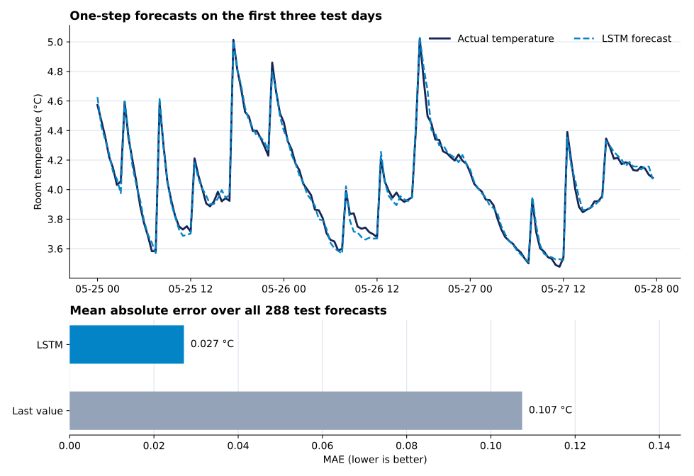
The upper panel shows that the forecast follows both gradual changes and short temperature rises. The lower panel summarizes all six test days, not only the visible three. Both methods receive the same target timestamps.

Shape the latest window for one new forecast

After training, a single live forecast still needs the batch dimension. Take the latest 12 scaled rows and add a leading dimension with reshape:

latest_window = torch.from_numpy(
    scaled_features[-lookback:].reshape(1, lookback, len(feature_names))
)

model.eval()
with torch.no_grad():
    next_scaled = model(latest_window).item()

next_prediction = next_scaled * target_std + target_mean
print("input shape:", tuple(latest_window.shape))
print(f"forecast: {next_prediction:.3f} °C")

input shape: (1, 12, 3)
forecast: 4.195 °C

The 1 means one sample, 12 means 12 ordered half-hour readings, and 3 means three features at each reading. The forecast is for 31 May 2025 at 00:00, one step after the final dataset row. No actual value is available for that timestamp, so this prediction cannot be scored yet.

In production, save the feature order with the model. A tensor with the correct shape but a different column order will run without an error and produce the wrong meaning.

Common mistakes and troubleshooting

Using (samples, features, timesteps). With batch_first=True, PyTorch expects (samples, timesteps, features). Print the tensor shape before training and connect every number to a meaning.

Setting input_size to the lookback. input_size is the feature count at one timestep. For this lesson it is 3. The lookback of 12 belongs in the sequence dimension.

Including the target inside its input window. A slice such as features[target_row - lookback:target_row + 1] includes the target row. End the slice at target_row, and inspect one boundary in original units.

Splitting completed windows by array percentage. This can move the test boundary away from the intended target timestamp. Keep the target row positions, then split with target_rows < test_start_row.

Fitting the scaler on all rows. Test-period statistics then influence training. Fit means and standard deviations on earlier rows only, and reuse them for validation, testing, and live inputs.

Dropping the batch dimension for one forecast. A single sample begins as (12, 3), but the model expects (1, 12, 3). Use reshape, np.newaxis, or PyTorch’s unsqueeze(0) to add it.

Shuffling individual timestamps. You may shuffle complete training windows, but never shuffle the 12 timesteps inside a window. Their order carries the sequence information.

Reporting training loss as forecast quality. Training loss is calculated on data used to update the model. Evaluate later targets and compare with a simple baseline on the same rows.

Assuming a longer window is automatically better. A longer lookback removes more early samples, costs more computation, and may add irrelevant history. Choose an initial length from the process timing, then compare alternatives on validation periods rather than the final test.

Treating synthetic accuracy as operational evidence. The generated data are intentionally learnable. Real sensors can drift, fail, or respond to events that are missing from the features. Rebuild the evaluation around real collection and decision timing before deployment.

Recap and next steps

An LSTM forecast begins with correct data alignment. For batch_first=True, the durable shape is (samples, timesteps, features). Each sample contains only past rows, and its target is the next value outside that window.

The complete workflow is:

1. Sort and verify the time grid.
2. Reserve a later period for testing.
3. Fit scaling statistics on earlier rows only.
4. Turn fixed-length histories into three-dimensional windows.
5. Split windows by their target timestamps.
6. Set input_size to the number of features.
7. Train on batches without changing timestep order.
8. Reverse the scaling and compare later forecasts with a baseline.

In this lesson, 12 half-hour steps and 3 features produced training inputs with shape (1140, 12, 3). The same pipeline produced 288 later forecasts. The LSTM reached 0.027 °C MAE, compared with 0.107 °C for the last-value baseline on this synthetic dataset.

As a next step, add a validation period between training and testing. Use it to compare two lookback lengths, such as 6 and 12 steps, while leaving the final six test days untouched. That separation lets you choose a window length without tuning to the numbers used for the final report.