Using Spark SQL in PySpark: Query DataFrames with Familiar SQL Syntax

PySpark gives you two ways to work with distributed data: the DataFrame API (.select(), .filter(), .groupBy()) and Spark SQL, where you write literal SELECT statements against registered views. If you already know SQL, Spark SQL is often the faster path to an answer — no new method names to memorize, no wondering which argument is col and which is a string. You just write the query.

This guide shows you how to register DataFrames as SQL views, run queries, join tables, aggregate with GROUP BY, and mix SQL with DataFrame transformations in the same pipeline. If you’re new to PySpark entirely, our PySpark for Beginners tutorial covers installation and the core DataFrame operations first.

The Mental Model: One Plan, Two Syntaxes

A SELECT statement and a chain of .filter()/.groupBy() calls look like different tools, but underneath they go through the same three steps:

1. Parse. Whatever syntax you wrote — a SQL string or a method chain — gets turned into a logical plan: a description of what you want, not data that’s actually been touched yet.
2. Optimize. Spark’s Catalyst optimizer rewrites that plan for efficiency. It doesn’t know or care whether the plan came from SQL or from DataFrame methods — by this point, they look identical to it.
3. Execute. Only when you call an action like .show() or .collect() does Spark actually read data and run the plan across its partitions.

A createOrReplaceTempView() call doesn’t copy or move anything either — it just gives Spark’s internal catalog a name to point at an existing DataFrame, so spark.sql() has something to reference by that name.

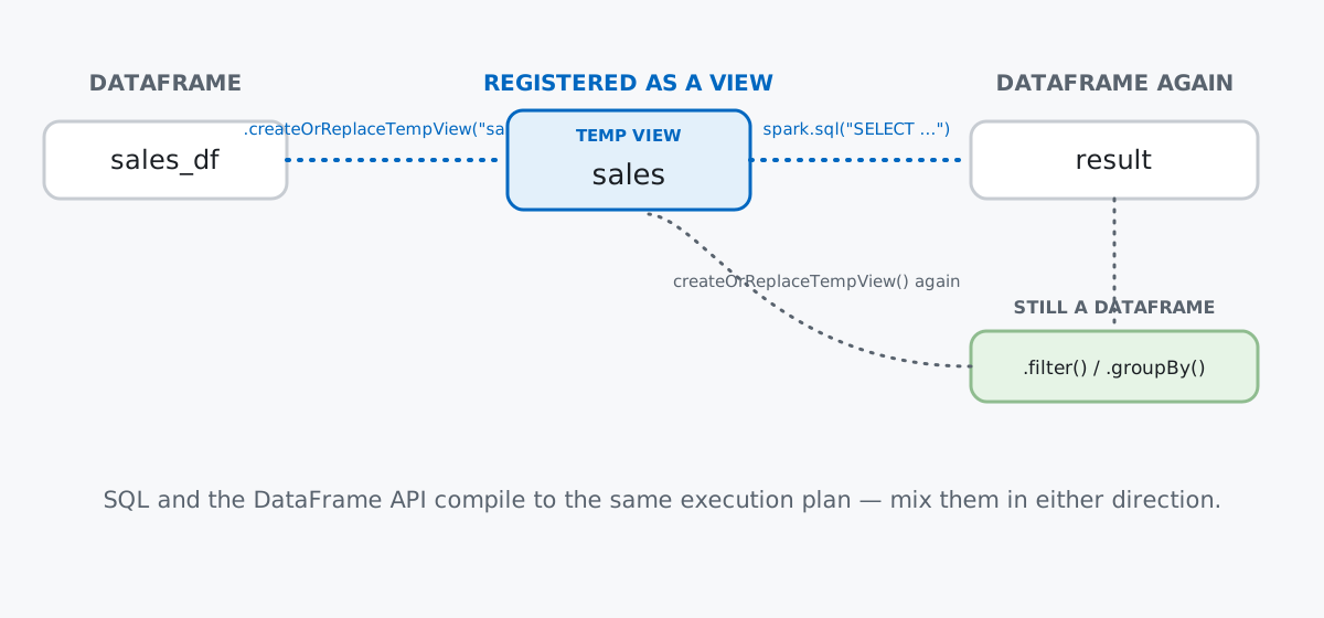
Keep that in mind for everything below: switching between SQL and the DataFrame API mid-pipeline costs nothing, because you’re only ever choosing which syntax to describe the same plan in.

Setting Up: DataFrames and Views

First, let’s create a Spark session and generate some sample data. We’ll use a small sales dataset:

from pyspark.sql import SparkSession

spark = SparkSession.builder \
    .appName("SparkSQLDemo") \
    .getOrCreate()

# Sample sales data
sales_data = [
    (1, "2024-01-15", "Alice", "Laptop", 1200, 1),
    (2, "2024-01-16", "Bob", "Mouse", 25, 2),
    (3, "2024-01-16", "Alice", "Keyboard", 75, 1),
    (4, "2024-01-17", "Charlie", "Monitor", 300, 2),
    (5, "2024-01-17", "Bob", "Laptop", 1200, 1),
    (6, "2024-01-18", "Alice", "Mouse", 25, 3),
    (7, "2024-01-18", "Charlie", "Keyboard", 75, 2),
]

columns = ["order_id", "date", "customer", "product", "price", "quantity"]
sales_df = spark.createDataFrame(sales_data, columns)

sales_df.show()

+--------+----------+--------+--------+-----+--------+
|order_id|      date|customer| product|price|quantity|
+--------+----------+--------+--------+-----+--------+
|       1|2024-01-15|   Alice|  Laptop| 1200|       1|
|       2|2024-01-16|     Bob|   Mouse|   25|       2|
|       3|2024-01-16|   Alice|Keyboard|   75|       1|
|       4|2024-01-17| Charlie| Monitor|  300|       2|
|       5|2024-01-17|     Bob|  Laptop| 1200|       1|
|       6|2024-01-18|   Alice|   Mouse|   25|       3|
|       7|2024-01-18| Charlie|Keyboard|   75|       2|
+--------+----------+--------+--------+-----+--------+

(The outputs in this post come from PySpark 3.5.3 on Python 3.11 — the same pinned version used in the PySpark for Beginners guide, since a plain pip install pyspark currently grabs 4.x, which needs a newer JDK than many machines have installed.)

To query this DataFrame with SQL, register it as a temporary view:

sales_df.createOrReplaceTempView("sales")

Now sales acts like a SQL table name — but it’s just a pointer to the DataFrame. The data stays in Spark’s distributed memory.

Your First SQL Query

Use spark.sql() to run a query. It returns a new DataFrame:

result = spark.sql("""
    SELECT customer, product, price * quantity AS total
    FROM sales
    WHERE price > 50
""")

result.show()

+--------+--------+-----+
|customer| product|total|
+--------+--------+-----+
|   Alice|  Laptop| 1200|
|   Alice|Keyboard|   75|
| Charlie| Monitor|  600|
|     Bob|  Laptop| 1200|
| Charlie|Keyboard|  150|
+--------+--------+-----+

Everything you know about SQL works: WHERE filters, AS aliases, column expressions. The query returns a DataFrame, so you can chain more operations:

result.filter(result.total > 100).show()

+--------+--------+-----+
|customer| product|total|
+--------+--------+-----+
|   Alice|  Laptop| 1200|
| Charlie| Monitor|  600|
|     Bob|  Laptop| 1200|
| Charlie|Keyboard|  150|
+--------+--------+-----+

You can switch between SQL and DataFrame methods freely — they’re two interfaces to the same underlying execution plan.

Aggregations with GROUP BY

How much did each customer spend in total?

customer_totals = spark.sql("""
    SELECT 
        customer,
        SUM(price * quantity) AS total_spent,
        COUNT(*) AS order_count
    FROM sales
    GROUP BY customer
    ORDER BY total_spent DESC
""")

customer_totals.show()

+--------+-----------+-----------+
|customer|total_spent|order_count|
+--------+-----------+-----------+
|   Alice|       1350|          3|
|     Bob|       1250|          2|
| Charlie|        750|          2|
+--------+-----------+-----------+

Alice leads with 3 orders totaling $1,350. The ORDER BY sorts within Spark’s distributed execution — it works the same as in Postgres or MySQL.

Joining Tables

Let’s add a customer info table and join it with sales:

customer_data = [
    ("Alice", "[email protected]", "New York"),
    ("Bob", "[email protected]", "San Francisco"),
    ("Charlie", "[email protected]", "Austin"),
]

customer_df = spark.createDataFrame(customer_data, ["name", "email", "city"])
customer_df.createOrReplaceTempView("customers")

customer_df.show()

+-------+-------------------+-------------+
|   name|              email|         city|
+-------+-------------------+-------------+
|  Alice|  [email protected]|     New York|
|    Bob|    [email protected]|San Francisco|
|Charlie|[email protected]|       Austin|
+-------+-------------------+-------------+

Now join them to see each order with customer details:

joined = spark.sql("""
    SELECT 
        s.order_id,
        s.date,
        c.name,
        c.city,
        s.product,
        s.price * s.quantity AS total
    FROM sales s
    INNER JOIN customers c ON s.customer = c.name
    ORDER BY s.date, s.order_id
""")

joined.show()

+--------+----------+-------+-------------+--------+-----+
|order_id|      date|   name|         city| product|total|
+--------+----------+-------+-------------+--------+-----+
|       1|2024-01-15|  Alice|     New York|  Laptop| 1200|
|       2|2024-01-16|    Bob|San Francisco|   Mouse|   50|
|       3|2024-01-16|  Alice|     New York|Keyboard|   75|
|       4|2024-01-17|Charlie|       Austin| Monitor|  600|
|       5|2024-01-17|    Bob|San Francisco|  Laptop| 1200|
|       6|2024-01-18|  Alice|     New York|   Mouse|   75|
|       7|2024-01-18|Charlie|       Austin|Keyboard|  150|
+--------+----------+-------+-------------+--------+-----+

Standard SQL joins — INNER, LEFT, RIGHT, FULL OUTER — all work. Spark optimizes the join execution across partitions automatically.

Window Functions

Rank each customer’s orders by total amount:

ranked = spark.sql("""
    SELECT 
        customer,
        product,
        price * quantity AS total,
        RANK() OVER (PARTITION BY customer ORDER BY price * quantity DESC) AS rank
    FROM sales
""")

ranked.show()

+--------+--------+-----+----+
|customer| product|total|rank|
+--------+--------+-----+----+
|   Alice|  Laptop| 1200|   1|
|   Alice|Keyboard|   75|   2|
|   Alice|   Mouse|   75|   2|
|     Bob|  Laptop| 1200|   1|
|     Bob|   Mouse|   50|   2|
| Charlie| Monitor|  600|   1|
| Charlie|Keyboard|  150|   2|
+--------+--------+-----+----+

Alice’s laptop purchase ranks first; her keyboard and mouse tie at second. Window functions (RANK, ROW_NUMBER, LAG, LEAD) work exactly as they do in traditional SQL databases — Spark’s SQL window function syntax reference lists the full set if you want to go beyond RANK.

Creating New Tables from Queries

Save a query result as a new view for reuse:

spark.sql("""
    CREATE OR REPLACE TEMP VIEW high_value_orders AS
    SELECT *
    FROM sales
    WHERE price * quantity > 100
""")

spark.sql("SELECT * FROM high_value_orders").show()

+--------+----------+--------+--------+-----+--------+
|order_id|      date|customer| product|price|quantity|
+--------+----------+--------+--------+-----+--------+
|       1|2024-01-15|   Alice|  Laptop| 1200|       1|
|       4|2024-01-17| Charlie| Monitor|  300|       2|
|       5|2024-01-17|     Bob|  Laptop| 1200|       1|
|       7|2024-01-18| Charlie|Keyboard|   75|       2|
+--------+----------+--------+--------+-----+--------+

Temporary views last for the session. If you want persistent tables, write to Parquet or Delta Lake instead:

result.write.mode("overwrite").parquet("/path/to/output")

Mixing SQL and DataFrame APIs

You don’t have to choose one approach for an entire pipeline. Start with SQL, switch to DataFrame methods when needed:

# Start with SQL
base = spark.sql("SELECT customer, price * quantity AS total FROM sales")

# Continue with DataFrame API
from pyspark.sql.functions import col

filtered = base.filter(col("total") > 100) \
               .groupBy("customer") \
               .sum("total") \
               .withColumnRenamed("sum(total)", "grand_total")

filtered.show()

+--------+-----------+
|customer|grand_total|
+--------+-----------+
|   Alice|       1200|
| Charlie|        750|
|     Bob|       1200|
+--------+-----------+

Or go the other direction: build a DataFrame pipeline, register it as a view, then query it:

df_result = sales_df.filter(col("price") > 50)
df_result.createOrReplaceTempView("expensive_items")

spark.sql("SELECT customer, COUNT(*) FROM expensive_items GROUP BY customer").show()

+--------+--------+
|customer|count(1)|
+--------+--------+
|   Alice|       2|
| Charlie|       2|
|     Bob|       1|
+--------+--------+

Use whichever syntax makes the logic clearer for that step.

When to Use SQL vs. DataFrame API

Use Spark SQL when:

• You already know the query in SQL and translating it to DataFrame methods would take longer
• You’re working with complex joins, subqueries, or window functions that are clearer in SQL syntax
• You’re collaborating with analysts or data engineers who think in SQL
• The query logic is easier to read as a single SELECT statement

Use the DataFrame API when:

• You’re building dynamic queries where column names or filters come from variables
• You want IDE autocomplete and type checking (SQL is just a string)
• The transformation is simpler as method chains (e.g., a quick .withColumn())
• You’re integrating with Python libraries that expect DataFrames

Both compile to the same Catalyst optimizer, so performance is identical — it’s purely about readability and workflow.

Performance Considerations

Spark SQL queries go through the same optimization as DataFrame API calls. The Catalyst optimizer rewrites your query plan regardless of syntax. A few things to keep in mind:

• Predicate pushdown works in both. WHERE filters in SQL and .filter() in DataFrames both push down to the data source when possible.
• Caching helps repeated queries. If you’re querying the same view multiple times, cache it: sales_df.cache() or spark.sql("CACHE TABLE sales").
• Avoid SELECT * on wide tables. Only select the columns you need — Spark’s columnar storage skips unread columns entirely.

Three Gotchas Worth Knowing

A typo in a SQL string fails the instant you call spark.sql() — you don’t need to wait for .show(). DataFrame method calls are lazy end to end, but spark.sql() parses and resolves your query against the catalog immediately, so a misspelled column raises before any action runs:

spark.sql("SELECT customr FROM sales").show()

pyspark.errors.exceptions.captured.AnalysisException: [UNRESOLVED_COLUMN.WITH_SUGGESTION] A column or function parameter with name `customr` cannot be resolved. Did you mean one of the following? [`customer`, `date`, `price`, `quantity`, `product`].

Spark even suggests the column you probably meant. Compare that to a DataFrame typo like sales_df.select("customr"), which raises the same kind of error — the difference is that a SQL string has no autocomplete to catch it before you run it at all.

A createOrReplaceTempView() name only lives for the current SparkSession — it won’t survive a notebook restart or a second session. If you need a view to outlive the session that created it, register it as a global temp view instead, and query it through the special global_temp database:

sales_df.createGlobalTempView("global_sales")
spark.sql("SELECT COUNT(*) FROM global_temp.global_sales").show()

+--------+
|count(1)|
+--------+
|       7|
+--------+

Querying it by its bare name, the way you would a regular temp view, fails — the global_temp prefix isn’t optional:

spark.sql("SELECT COUNT(*) FROM global_sales").show()

pyspark.errors.exceptions.captured.AnalysisException: [TABLE_OR_VIEW_NOT_FOUND] The table or view `global_sales` cannot be found.

Joining a table to itself (or to another table with overlapping column names) makes a bare column name ambiguous, and Spark refuses to guess. Self-joins are common enough — comparing each order against other orders of the same product, say — that this is worth expecting rather than being surprised by:

spark.sql("""
    SELECT customer, product
    FROM sales s1
    JOIN sales s2 ON s1.product = s2.product
""").show()

pyspark.errors.exceptions.captured.AnalysisException: [AMBIGUOUS_REFERENCE] Reference `customer` is ambiguous, could be: [`s1`.`customer`, `s2`.`customer`].

Qualify the column with its table alias — s1.customer — and the ambiguity goes away. This is the same rule as the joins you wrote earlier: it only stayed invisible there because sales and customers didn’t happen to share a column name.

Wrapping Up

Spark SQL lets you query PySpark DataFrames with standard SQL: register a DataFrame as a temporary view with .createOrReplaceTempView(), run queries with spark.sql(), and get back a DataFrame you can keep transforming. Joins, aggregations, window functions, and subqueries all work as expected. Mix SQL and DataFrame API calls freely — they’re two ways to express the same distributed execution plan.

If you want to go deeper on the SQL side of this — window functions, subqueries, CTEs, and query optimization on a real database rather than a distributed engine — the Window Functions lessons in our free SQL & Databases course pick up exactly where the RANK() example above leaves off. And if PySpark itself is still new to you, PySpark for Beginners covers the DataFrame API, lazy evaluation, and installation from scratch.