Wrangling Survey Data with Pandas: A Star Wars Case Study

A spreadsheet export from a survey tool almost never looks like the tables you practiced pandas on. One question becomes one column (“Are you a fan?”). Another question becomes six columns, one per checkbox, because the respondent could pick more than one answer. A third becomes six more columns, each holding a number from 1 to 6, because the respondent had to rank every option. Load all of that with pd.read_csv() and default settings, and you get a DataFrame that’s technically loaded but not actually usable yet.

This is where a lot of people either give up and start manually re-typing column names, or plow ahead and quietly get the wrong answer — because a blank cell means something different depending on which of those three question shapes it’s sitting in. (If messy-data cleaning in general is new to you, our guide to cleaning messy data with pandas covers the broader detect-decide-fix workflow; this post is about the specific shapes survey exports produce.) We’ll fix all of it, end to end, using a real public dataset: FiveThirtyEight’s 2014 survey of over 1,000 Star Wars fans.

The Mental Model: Three Answer Shapes

Before touching any code, it helps to recognize that almost every question in a raw survey export takes one of three shapes:

1. Single-choice. One question, one column, one value per respondent (“Do you consider yourself a fan?” → Yes / No).
2. Multi-select (“select all that apply”). One question, spread across several columns — one column per option — where a filled cell means “picked” and a blank cell means “not picked.” Nothing here is actually missing data.
3. Forced rank. One question, again spread across several columns — one column per item being ranked — where every cell holds a number (1st place, 2nd place, and so on) instead of a label.

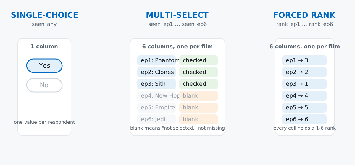
Once you know which shape you’re looking at, the cleaning step is obvious: single-choice columns just need value_counts(), multi-select columns need a blank-to-boolean conversion, and rank columns need you to think carefully about who was actually eligible to rank before you average anything. We’ll do all three below.

A Dataset You Can Reproduce

FiveThirtyEight ran a reader survey in 2014 that asked over 1,000 U.S. respondents whether they’d seen each Star Wars film, how they’d rank the six films, and how they felt about fourteen characters. The raw export is a genuinely messy real file — a two-row header, Windows-1252 characters that break UTF-8 decoding, and real skip logic — which makes it a good stand-in for what a survey tool actually hands you.

Data: the 2014 Star Wars fan survey (CC BY 4.0), via FiveThirtyEight’s public data repository. Grab your own copy at /datasets/blog/star-wars-survey-pandas/StarWarsSurvey.csv to follow along with the exact numbers below.

Try loading it the obvious way first:

import pandas as pd

pd.read_csv("StarWarsSurvey.csv", encoding="utf-8", nrows=5)

UnicodeDecodeError: 'utf-8' codec can't decode byte 0x8c in position 62: invalid start byte

The file was exported with a Windows-1252-family encoding, not UTF-8. encoding="latin-1" reads any byte value without raising, which is the pragmatic fix for old survey exports like this one. (The outputs in this post come from pandas 3.0.3 — everything shown also works on pandas 2.x.)

Turning Two Header Rows into One Clean Column List

Open the raw file and rows 1 and 2 are both headers: row 1 has the full question text (repeated across every column that question spans, or blank where it doesn’t apply), and row 2 has the specific sub-label — a film title, a character name, or just “Response.” Neither row alone is a usable column name, and pandas’ header=[0, 1] multi-index option just hands you both rows glued together, unnamed gaps and all.

The more direct fix: since we already know the shape of this survey (three demographic-style questions, six seen-columns, six rank-columns, fourteen favorability-columns, and five more single-choice questions), skip both header rows and supply the column names ourselves.

column_names = [
    "respondent_id", "seen_any", "is_fan",
    "seen_ep1", "seen_ep2", "seen_ep3", "seen_ep4", "seen_ep5", "seen_ep6",
    "rank_ep1", "rank_ep2", "rank_ep3", "rank_ep4", "rank_ep5", "rank_ep6",
    "fav_han_solo", "fav_luke_skywalker", "fav_leia_organa", "fav_anakin_skywalker",
    "fav_obi_wan_kenobi", "fav_emperor_palpatine", "fav_darth_vader", "fav_lando_calrissian",
    "fav_boba_fett", "fav_c3po", "fav_r2d2", "fav_jar_jar_binks", "fav_padme_amidala", "fav_yoda",
    "shot_first", "familiar_expanded_universe", "fan_expanded_universe", "fan_star_trek",
    "gender", "age", "household_income", "education", "location_census_region",
]

survey = pd.read_csv(
    "StarWarsSurvey.csv",
    skiprows=2,
    header=None,
    names=column_names,
    encoding="latin-1",
)
survey.shape

(1186, 38)

skiprows=2 drops both header rows, header=None tells pandas not to treat the next row as a header either, and names= supplies our own list — which has to have exactly 38 entries to match the file’s 38 columns. See the full parameter list in the official read_csv docs if you want to go further than what this post covers. One respondent, spot-checked:

survey.loc[0, ["respondent_id", "seen_any", "is_fan", "seen_ep1", "rank_ep1", "fav_han_solo"]]

respondent_id                                  3292879998
seen_any                                              Yes
is_fan                                                Yes
seen_ep1         Star Wars: Episode I  The Phantom Menace
rank_ep1                                              3.0
fav_han_solo                               Very favorably
Name: 0, dtype: object

seen_ep1 and rank_ep1 are still in their raw shapes — a repeated title string and a float — which is exactly what we clean up next.

value_counts() and Skip Logic in Single-Choice Columns

seen_any and is_fan are the simplest shape: one question, one column, one answer.

survey["seen_any"].value_counts(dropna=False)

seen_any
Yes    936
No     250
Name: count, dtype: int64

936 of 1,186 respondents had seen at least one film. Check is_fan next and something looks off:

survey["is_fan"].value_counts()

is_fan
Yes    552
No     284
Name: count, dtype: int64

552 + 284 is 836, not 1,186. value_counts() drops NaN by default, and there are 350 respondents missing here. Pass dropna=False to see them:

survey["is_fan"].value_counts(dropna=False)

is_fan
Yes    552
NaN    350
No     284
Name: count, dtype: int64

Those 350 aren’t random nonresponse. This survey used skip logic: if you answered No to “have you seen any of the films,” the questionnaire never asked whether you’re a fan.

survey.loc[survey["seen_any"] == "No", "is_fan"].isna().sum()

250

All 250 people who hadn’t seen a film account for most of the 350 NaNs. The other 100 are respondents who had seen a film but still skipped the fan question — genuine nonresponse, not skip logic. Both look identical as NaN in the column, but they mean different things, which matters the moment you consider filling them in.

Checkbox Questions: .notna() Turns Blanks into Booleans

“Which films have you seen? Select all that apply” spans six columns, seen_ep1 through seen_ep6. In the raw export, a selected checkbox stores the film’s full title as text; an unselected one is blank:

survey[["seen_ep1", "seen_ep4"]].head(3)

                                   seen_ep1                           seen_ep4
0  Star Wars: Episode I  The Phantom Menace  Star Wars: Episode IV  A New Hope
1                                       NaN                                NaN
2  Star Wars: Episode I  The Phantom Menace                                NaN

That’s an unusual way to store a checkbox, but it converts cleanly: the presence of any value means “selected,” regardless of what the value says.

seen_cols = ["seen_ep1", "seen_ep2", "seen_ep3", "seen_ep4", "seen_ep5", "seen_ep6"]
for col in seen_cols:
    survey[col] = survey[col].notna()

survey[["seen_ep1", "seen_ep4"]].head(3)

   seen_ep1  seen_ep4
0      True      True
1     False     False
2      True     False

With six boolean columns, “how many people saw each film” is one line:

film_titles = {
    "ep1": "The Phantom Menace", "ep2": "Attack of the Clones", "ep3": "Revenge of the Sith",
    "ep4": "A New Hope", "ep5": "The Empire Strikes Back", "ep6": "Return of the Jedi",
}
survey[seen_cols].sum().rename(lambda c: film_titles[c.split("_")[1]]).sort_values(ascending=False)

The Empire Strikes Back    758
Return of the Jedi         738
The Phantom Menace         673
A New Hope                 607
Attack of the Clones       571
Revenge of the Sith        550
dtype: int64

.rename(lambda c: ...) swaps the internal seen_epN keys for readable titles right before display — the underlying data stays untouched. Notice the original trilogy (episodes IV-VI) isn’t a clean sweep over the prequels here; more people report having seen The Phantom Menace than Attack of the Clones.

Ranking Columns: .mean() Reveals the Fan Favorite

The six rank_epN columns hold each respondent’s 1-to-6 preference order — already numeric, no conversion needed:

rank_cols = ["rank_ep1", "rank_ep2", "rank_ep3", "rank_ep4", "rank_ep5", "rank_ep6"]
survey[rank_cols].dtypes

rank_ep1    float64
rank_ep2    float64
rank_ep3    float64
rank_ep4    float64
rank_ep5    float64
rank_ep6    float64
dtype: object

The naive move is to average each column straight away. Don’t do that yet — someone who never saw Attack of the Clones couldn’t rank it, and a NaN there just means pandas’ .mean() silently ignores it, averaging over whatever subset of respondents happened to rank that particular film. To compare films fairly, first restrict to people who ranked all six — meaning they’d seen all six:

saw_all_six = survey[seen_cols].all(axis=1)
saw_all_six.sum()

471

survey.loc[saw_all_six, rank_cols].mean().rename(lambda c: film_titles[c.split("_")[1]]).sort_values().round(2)

The Empire Strikes Back    2.38
A New Hope                 2.87
Return of the Jedi         2.93
The Phantom Menace         4.24
Revenge of the Sith        4.25
Attack of the Clones       4.33
dtype: float64

Among the 471 respondents who’d seen every film, The Empire Strikes Back wins comfortably (lower average rank is better — 1 was “favorite”), and the original trilogy sweeps the top three spots.

Character Favorability: Building a net_favorable Score

Fourteen more columns each hold a five-point favorability label per character, or "Unfamiliar (N/A)" if the respondent didn’t know them. A single net_favorable score — the share who rated a character favorably minus the share who rated them unfavorably, among people who expressed an opinion — makes fourteen columns comparable at a glance:

character_names = {
    "fav_han_solo": "Han Solo", "fav_luke_skywalker": "Luke Skywalker",
    "fav_leia_organa": "Leia Organa", "fav_anakin_skywalker": "Anakin Skywalker",
    "fav_obi_wan_kenobi": "Obi-Wan Kenobi", "fav_emperor_palpatine": "Emperor Palpatine",
    "fav_darth_vader": "Darth Vader", "fav_lando_calrissian": "Lando Calrissian",
    "fav_boba_fett": "Boba Fett", "fav_c3po": "C-3PO", "fav_r2d2": "R2-D2",
    "fav_jar_jar_binks": "Jar Jar Binks", "fav_padme_amidala": "Padme Amidala", "fav_yoda": "Yoda",
}
favorable = {"Very favorably", "Somewhat favorably"}
unfavorable = {"Very unfavorably", "Somewhat unfavorably"}
neutral = {"Neither favorably nor unfavorably (neutral)"}

rows = []
for col, name in character_names.items():
    opinion = survey[col].isin(favorable | unfavorable | neutral)
    pct_fav = round(survey.loc[opinion, col].isin(favorable).mean() * 100, 1)
    pct_unfav = round(survey.loc[opinion, col].isin(unfavorable).mean() * 100, 1)
    rows.append((name, opinion.sum(), pct_fav, pct_unfav, round(pct_fav - pct_unfav, 1)))

net_favorability = pd.DataFrame(
    rows, columns=["character", "n", "pct_favorable", "pct_unfavorable", "net_favorable"]
).sort_values("net_favorable", ascending=False).reset_index(drop=True)
net_favorability

            character    n  pct_favorable  pct_unfavorable  net_favorable
0            Han Solo  814           93.5              1.1           92.4
1      Luke Skywalker  825           93.5              1.9           91.6
2      Obi-Wan Kenobi  808           92.8              1.9           90.9
3         Leia Organa  823           92.0              2.2           89.8
4                Yoda  816           91.8              2.0           89.8
5               R2-D2  820           91.1              2.0           89.1
6               C-3PO  812           86.6              3.7           82.9
7    Anakin Skywalker  771           66.7             15.8           50.9
8    Lando Calrissian  672           54.3             10.6           43.7
9       Padme Amidala  650           54.0             14.2           39.8
10        Darth Vader  816           58.9             30.8           28.1
11          Boba Fett  680           42.8             20.7           22.1
12  Emperor Palpatine  658           38.4             29.2            9.2
13      Jar Jar Binks  712           34.0             43.0           -9.0

Deliberately excluding the "Unfamiliar (N/A)" respondents from the denominator matters: it means net_favorable measures opinion among people who have one, not “fame.” One character stands alone at the bottom with a negative score — Jar Jar Binks is the only one of the fourteen where more respondents with an opinion disliked him than liked him.

Four Gotchas Worth Knowing

The default encoding will fail on old survey exports. Most spreadsheet tools that export CSVs from before UTF-8 became universal used a Windows-1252-family encoding. pd.read_csv(path) assumes UTF-8 and raises UnicodeDecodeError the moment it hits a byte like 0x8c. encoding="latin-1" (or "cp1252") reads every byte value without raising — it’s the standard workaround, not a real character-set fix, but it’s fine for a numeric/text survey export like this one.

value_counts() hides how much skip logic is in play. Its default dropna=True means a quick .value_counts() on is_fan looks like a complete 836-respondent picture when 350 more respondents are sitting off-screen. Always check with dropna=False before you trust a percentage breakdown from survey data.

Not all NaN in the same column means the same thing. is_fan mixes 250 respondents who were never asked (skip logic, because they said No to “have you seen any films”) with 100 who were asked and didn’t answer (real nonresponse). Filling both with the same value — False, "No", or anything else — would misrepresent the 250 as having an opinion they were never asked for.

Averaging over the wrong subgroup quietly changes the answer. Skip the saw_all_six filter and average rank_epN over every respondent who ranked that film at all:

survey[rank_cols].mean().rename(lambda c: film_titles[c.split("_")[1]]).sort_values().round(2)

The Empire Strikes Back    2.51
Return of the Jedi         3.05
A New Hope                 3.27
The Phantom Menace         3.73
Attack of the Clones       4.09
Revenge of the Sith        4.34
dtype: float64

Return of the Jedi now edges out A New Hope for second place — the opposite of the order two sections ago. Nothing about the underlying opinions changed; only the eligible respondent set did, silently, because .mean() skips NaN without telling you who it skipped. Decide who’s eligible to answer a comparison before you average across it — the eligible subset isn’t always “everyone who has a value here.”

Wrapping Up

Every raw survey export reduces to three answer shapes: single-choice columns you can hand straight to value_counts(), multi-select columns where .notna() turns filled-vs-blank into True/False, and forced-rank columns where .mean() only means what you think it means once you’ve restricted to respondents who were actually eligible to answer. Add dropna=False to catch skip logic hiding in plain sight, and you can turn almost any questionnaire export into an analysis-ready DataFrame.

If you want more practice turning real, imperfect data into something analysis-ready, the Pandas Data Analysis lessons in our free Python for Data Analytics course build the same instincts — cleaning, reshaping, and aggregating — on several more datasets from scratch.