How to Stream a Large CSV into SQLite with Python

A CSV export can grow beyond the memory available to Python. Loading the entire file into one large list or DataFrame may then fail, even when you only need to count rows or filter one station.

This tutorial takes a different route: read one row at a time, collect a small batch, and insert that batch into an SQLite database on disk. SQLite is a database stored in a local file. It runs inside your Python process, so there is no database server to install. Once the import is complete, SQL can filter and summarize the data without loading every row into Python.

We will use fictional bicycle-counter readings. The complete example has 34,560 rows, which still runs quickly on a laptop. The same import pattern keeps only one fixed-size batch in memory, so it also applies to much larger files.

Prerequisites and setup

You need Python 3.10 or newer and basic knowledge of loops and functions. You do not need prior database experience. The import uses csv and sqlite3, which are included with Python. Matplotlib is needed only for the final chart.

Create a folder, open a terminal in it, and make a virtual environment:

python3 -m venv .venv
source .venv/bin/activate
python -m pip install matplotlib==3.11.0

On Windows PowerShell, activate the environment with .venv\Scripts\Activate.ps1 instead. The published output was tested with Python 3.13.2, SQLite 3.50.2, and Matplotlib 3.11.0.

Download the tutorial’s synthetic bicycle-counter CSV and save it beside your script. It is an original, deterministic teaching dataset released under CC0 1.0. The station names and all readings are fictional. This makes the example reproducible and avoids exposing real movement data.

The mental model: file, batch, database

A common mistake is to call list(reader) after opening a CSV. That consumes the iterator and creates a Python object for every row. Memory use then grows with the file.

Our pipeline has three smaller parts:

1. csv.DictReader yields one row at a time.
2. A batching function collects at most 2,000 rows.
3. SQLite writes each batch to an on-disk table.

An iterator is an object that supplies the next item only when requested. A batch is a limited group of rows handled together. If a file grows from 35,000 rows to 35 million rows, the batch still contains at most 2,000 rows. The database file grows, but the import batch does not.

SQLite is also a useful intermediate format. CSV has no data types, indexes, or query planner. A database table can reject negative counts, look up a time range, and calculate grouped totals directly.

Inspect the source before importing it

Start small. Open the CSV and print three rows before creating a database. This confirms the delimiter and column names.

import csv
from pathlib import Path

csv_path = Path("bicycle_counter_readings.csv")

with csv_path.open(newline="", encoding="utf-8") as handle:
    reader = csv.DictReader(handle)
    for _ in range(3):
        print(next(reader))

The real output begins like this:

{'reading_id': '1', 'recorded_at': '2026-01-01T00:00', 'station': 'Riverside', 'direction': 'inbound', 'bicycles': '19'}
{'reading_id': '2', 'recorded_at': '2026-01-01T00:00', 'station': 'Riverside', 'direction': 'outbound', 'bicycles': '30'}
{'reading_id': '3', 'recorded_at': '2026-01-01T00:00', 'station': 'Market Gate', 'direction': 'inbound', 'bicycles': '16'}

Every value is a string because CSV does not store type information. We will convert the ID and count to integers during import. Keeping recorded_at as ISO 8601 text is deliberate: values in YYYY-MM-DDTHH:MM order also sort in chronological order.

Create a table that checks incoming rows

Now connect to an on-disk database and create the destination table. A constraint is a rule the database applies before accepting a row. These constraints reject missing fields, an unexpected direction, and negative bicycle counts.

import sqlite3

database_path = Path("bicycle_counters.db")
database_path.unlink(missing_ok=True)
connection = sqlite3.connect(database_path)

connection.execute("""
    CREATE TABLE readings (
        reading_id INTEGER PRIMARY KEY,
        recorded_at TEXT NOT NULL,
        station TEXT NOT NULL,
        direction TEXT NOT NULL
            CHECK (direction IN ('inbound', 'outbound')),
        bicycles INTEGER NOT NULL CHECK (bicycles >= 0)
    )
""")

PRIMARY KEY makes every reading_id unique. NOT NULL prevents a missing value. These checks turn some silent data problems into clear errors during the import.

Stream and insert fixed-size batches

The next function takes any iterable object and yields lists of at most size items. An iterable is something Python can loop over. Here, it is the generator that converts CSV rows. islice takes only the next size items instead of consuming the rest of the file.

from itertools import islice

def batched(rows, size):
    iterator = iter(rows)
    while batch := list(islice(iterator, size)):
        yield batch

Next, reopen the CSV and transform each dictionary into a tuple that matches the table’s column order. The expression in parentheses creates a generator, an iterator that produces one converted tuple at a time. It does not build a second copy of the file in memory.

batch_size = 2_000
batches = 0

with csv_path.open(newline="", encoding="utf-8") as handle:
    reader = csv.DictReader(handle)
    rows = (
        (
            int(row["reading_id"]),
            row["recorded_at"],
            row["station"],
            row["direction"],
            int(row["bicycles"]),
        )
        for row in reader
    )

    with connection:
        for batch in batched(rows, batch_size):
            connection.executemany(
                "INSERT INTO readings VALUES (?, ?, ?, ?, ?)",
                batch,
            )
            batches += 1

row_count = connection.execute(
    "SELECT COUNT(*) FROM readings"
).fetchone()[0]
print(f"imported {row_count:,} rows in {batches} batches")

imported 34,560 rows in 18 batches

executemany calls the same parameterized SQL statement once for every tuple. The question marks are placeholders. Python binds each value safely and handles quoting; do not construct an INSERT with an f-string. The Python sqlite3 documentation recommends placeholders and shows the same executemany pattern.

The with connection: block is a transaction boundary. A transaction treats the inserts as one unit: it commits them if the block succeeds and rolls them back if an exception reaches the block. It does not close the connection.

The final batch contains only 560 rows. That is fine: islice returns the remaining items, and the next call returns an empty list and stops the loop.

How to choose a batch size

There is no universal best batch size. A batch of 2,000 works well for this example because it avoids one database call per row while remaining easy to hold in memory. Start with a few thousand rows, measure the import on your own machine, and adjust only when there is a reason.

A larger batch reduces the number of calls to SQLite, but each batch uses more memory. The effect depends on row width: 2,000 short numeric rows are much smaller than 2,000 rows containing long text documents. A smaller batch is safer when rows contain large strings or when the process has a strict memory limit. Avoid treating the batch size as a performance promise; storage speed, constraints, indexes, and transaction boundaries also affect import time.

Ask SQL for a compact result

The database can now summarize all 34,560 rows while Python receives only four result rows. This query groups readings by station and calculates a total and a mean.

connection.row_factory = sqlite3.Row

summary = connection.execute("""
    SELECT station,
           SUM(bicycles) AS total_bicycles,
           ROUND(AVG(bicycles), 1) AS mean_per_reading
    FROM readings
    GROUP BY station
    ORDER BY total_bicycles DESC
""").fetchall()

for row in summary:
    print(dict(row))

{'station': 'Riverside', 'total_bicycles': 450799, 'mean_per_reading': 52.2}
{'station': 'University', 'total_bicycles': 410559, 'mean_per_reading': 47.5}
{'station': 'Market Gate', 'total_bicycles': 357754, 'mean_per_reading': 41.4}
{'station': 'North Bridge', 'total_bicycles': 304056, 'mean_per_reading': 35.2}

Read the first row as follows: Riverside recorded 450,799 fictional bicycle passages across both directions and 180 days. The mean was 52.2 bicycles per reading, where each reading represents one direction during one hour. The total does not represent 450,799 unique people; one person may pass a counter more than once.

If grouped queries are new, the Pandas GroupBy tutorial explains the same split, calculate, and combine idea with a DataFrame.

Add an index for repeated lookups

An index is a separate lookup structure that helps SQLite find matching rows without checking the whole table. It costs disk space and adds work to inserts because SQLite must update both the table and the index. For a one-time import, load and validate the rows first, then add the indexes that real queries need. Keeping the index is usually reasonable for later small updates.

Our repeated question filters first by station and then by a timestamp range. Put the columns in that order in one compound index:

connection.execute("""
    CREATE INDEX idx_readings_station_time
    ON readings(station, recorded_at)
""")
connection.commit()

Use placeholders again for the filter values:

may_total = connection.execute("""
    SELECT SUM(bicycles)
    FROM readings
    WHERE station = ?
      AND recorded_at >= ?
      AND recorded_at < ?
""", ("University", "2026-05-01", "2026-06-01")).fetchone()[0]

print(may_total)

80779

The upper boundary uses < '2026-06-01', not an assumed final time on May 31. This half-open range includes every May timestamp, even if the file later gains seconds or fractional seconds.

EXPLAIN QUERY PLAN gives a short description of SQLite’s strategy:

plan = connection.execute("""
    EXPLAIN QUERY PLAN
    SELECT SUM(bicycles) FROM readings
    WHERE station = ? AND recorded_at >= ? AND recorded_at < ?
""", ("University", "2026-05-01", "2026-06-01")).fetchone()[3]

print(plan)

SEARCH readings USING INDEX idx_readings_station_time (station=? AND recorded_at>? AND recorded_at<?)

SEARCH ... USING INDEX confirms that this tested SQLite version chose the new index. The official SQLite query-plan guide warns that the exact text can change between releases, so use this output for inspection, not as a format your application parses.

Plot a small SQL result, not the full file

For the chart, let SQLite reduce the table to seven weekday totals. Only those seven numbers move into Python. SQLite’s strftime('%w', ...) returns Sunday as 0 through Saturday as 6.

weekday_rows = connection.execute("""
    SELECT CAST(strftime('%w', recorded_at) AS INTEGER) AS weekday,
           SUM(bicycles) AS bicycles
    FROM readings
    GROUP BY weekday
    ORDER BY weekday
""").fetchall()

connection.close()

Before importing pyplot, select the non-interactive Agg backend. This lets the script run on a server without a display.

import matplotlib
matplotlib.use("Agg")
import matplotlib.pyplot as plt

labels = ["Sun", "Mon", "Tue", "Wed", "Thu", "Fri", "Sat"]
values = [row["bicycles"] for row in weekday_rows]

fig, ax = plt.subplots(figsize=(9.2, 5.2))
ax.bar(labels, values)
ax.set_title("Weekday commuting produces the highest bicycle counts")
ax.set_ylabel("Bicycles across 180 days")
fig.tight_layout()
fig.savefig("weekday-profile.svg")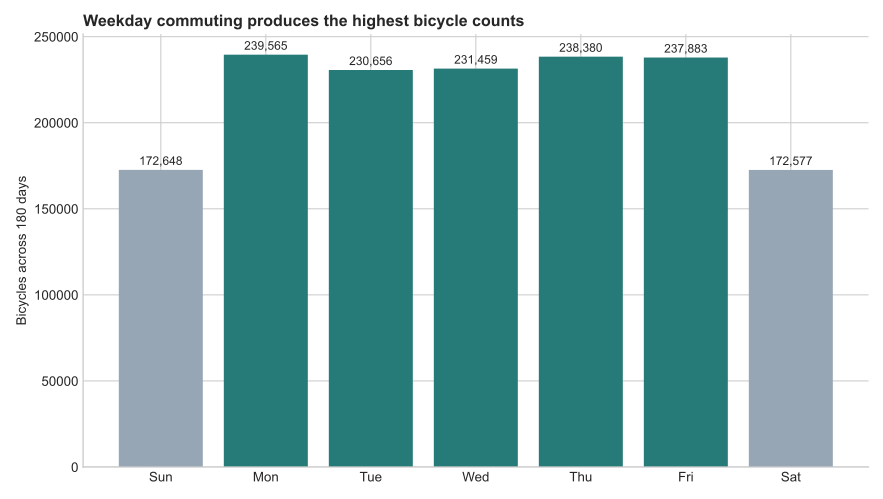

The Monday-to-Friday bars are higher because the synthetic generator includes morning and evening commuting peaks on those days. This result checks the data-generation rule; it is not evidence about a real city.

Common mistakes and troubleshooting

The script still uses too much memory. Check that you did not write list(csv.DictReader(handle)) or combine all batches after reading them. Only the current batch should become a list. Reduce batch_size if each row contains large text fields.

You get ValueError: invalid literal for int(). A numeric field contains text or an empty string. Print the current row inside a temporary try/except block to find it. Decide whether to reject, repair, or record bad rows; silently converting them to zero changes the meaning of the data.

You get sqlite3.IntegrityError. A row broke a table constraint, often because an ID was duplicated or a count was negative. This is useful validation. Inspect the offending batch instead of removing the constraint.

The database contains rows from an earlier run. Delete the old database before recreating it, as this tutorial does, or use a deliberate update strategy. Re-running plain inserts against the same table can duplicate data or violate the primary key.

The query plan says SCAN readings. Confirm that the index exists and that the filter starts with station, the first index column. For a small table SQLite may still decide a scan is cheaper. The planner, not the presence of an index alone, chooses the strategy.

The database is locked. Another process may have an open write transaction. Close unused connections, keep transactions focused, and avoid leaving a debugger paused inside a write block.

Recap

The durable pattern is simple: keep the large file on disk, iterate through it, convert only the current row, and insert fixed-size batches inside a transaction. Then let SQL reduce the full table to the small result Python actually needs.

You also added validation with table constraints, verified the imported row count, created a compound index after the bulk load, checked that SQLite used it, and plotted only seven aggregated values. This approach does not make every large-data problem an SQLite problem, but it is a practical next step when a CSV no longer fits comfortably in memory and one machine is still enough.